Backwardation
逆ザヤ Forward Curve ✓ Verified Citations Academic Origin<Mechanism>
Backwardation is not merely a price inversion; it is a price structure that reflects the market's underlying supply-demand condition. Three closely related factors sit behind it: inventory levels, the benefit of holding physical inventory, and futures price formation.
When inventories are ample, the additional value of holding physical supply is relatively small. As inventories decline and spare supply capacity falls, the value of having physical product immediately available rises.
As inventory falls, the benefit of holding physical inventory available for immediate use tends to rise, pushing up the convenience yield.
When this yield exceeds storage and financing costs, the physical commodity available today is valued more highly than the physical commodity to be delivered in the future.
As a result, the near-month price rises above the deferred-month price — backwardation.
This framework traces back to Keynes's (1930) Normal Backwardation hypothesis (the risk-premium theory). Kaldor (1939) then organized the concept of convenience yield, and Working (1933, 1949) systematized it as the Theory of Storage. Brennan (1958) further extended this into a supply-of-storage model and cost-of-carry theory.
<Example> A quantitatively and symbolically representative episode of backwardation in the WTI crude futures market was observed immediately after Russia's invasion of Ukraine in March 2022. At the time, OECD commercial crude inventories were trading below their five-year average, and this coincided with supply-disruption fears, pushing up the value of immediately available crude and producing a strong backwardation in which the near-month price traded well above the deferred-month price (EIA, 2022). CME Group's NYMEX WTI Futures Settlement Data shows the futures curve moving sharply into backwardation during this period. In this environment, investors rolling positions forward by successively closing near-month contracts and moving into deferred months found themselves selling the (expensive) near-month and buying the (cheaper) deferred month — a structure that generated positive roll yield independent of the underlying spot price movement itself. This episode became a landmark empirical example of how a sharp drawdown in physical inventory can steepen the slope (spread) of the futures curve.
<Issues and Caveats>
1. The unmeasurability and residual nature of convenience yield — Convenience yield is calculated as a residual (a byproduct of the model) derived by subtracting interest rates and storage costs from the price differential (spread) between the spot and futures markets. Because it has no directly observable market transaction price (it is unmeasurable), it is difficult to rigorously separate whether the resulting value reflects the genuine physical convenience of holding the commodity, or instead reflects market frictions, liquidity constraints, or temporary price distortions that the model does not capture — this remains an academic challenge.
2. A caveat on positive roll yield: the risk of reversal into contango — Under backwardation, rolling a position from the near month into the deferred month can generate a positive roll yield, but this effect changes as the shape of the curve changes. If the market structure shifts into contango — driven by a build-up in physical inventory or the easing of supply constraints — the roll yield that had been generating gains can flip to negative (a negative roll) almost immediately. Investors must therefore continuously assess the risk that the direction of the spread reverses as the market structure changes (a regime shift).
3. Keynes's theory (the Normal Backwardation hypothesis) and its scope of application — The risk-premium theory Keynes (1930) proposed — the so-called Normal Backwardation hypothesis — explains the possibility that futures prices are discounted relative to the expected future spot price, driven by producers' hedging demand. Subsequent work, however — Working's (1949) theory of storage and Brennan's (1958) cost-of-carry theory — showed that inventory levels, convenience yield, and storage costs also play an important role in shaping the futures curve. When assessing what drives backwardation, it is preferable to interpret it through multiple theoretical frameworks rather than a single theory alone.
- Keynes, J.M. (1930) "A Treatise on Money" (Vol. II) — Proposed the theory of Normal Backwardation, arguing that the persistent excess of producers' short-hedging demand discounts futures prices
- Working, H. (1933) "Price Relations between July and September Wheat Futures at Chicago Since 1885" — The origin of the Theory of Storage, developed by Holbrook Working starting in 1933 and later summarized in his 1948 and 1949 papers
- Kaldor, N. (1939) "Speculation and Economic Stability" (Review of Economic Studies, Vol.7, No.1, pp.1-27) — Extended by Nicholas Kaldor in 1939, introducing the concept of convenience yield
- Working, H. (1949) "The Theory of Price of Storage" (American Economic Review) — Systematized the Theory of Storage
- Brennan, M.J. (1958) "The Supply of Storage" (American Economic Review) — Further extended by Brennan in 1958 through estimation of demand and supply curves for storage
- Fama, E.F., & French, K.R. (1987) "Commodity Futures Prices: Some Evidence on Forecast Power, Premiums, and the Theory of Storage" (Journal of Business, Vol.60, No.1, pp.55-73) — Empirically demonstrated the residual nature of convenience yield within the cost-of-carry model
- CME Group (2022) "NYMEX WTI Crude Futures Settlement Prices," CME Group — Settlement price data source showing the WTI futures curve's shift into backwardation in March 2022
- EIA (2022) "Petroleum & Other Liquids Data / U.S. Ending Stocks of Crude Oil," U.S. Energy Information Administration — Official data source for March 2022 WTI inventory levels
Contango
順ザヤ Forward Curve ✓ Verified Citations Academic Origin<Mechanism>
Contango is not merely a normal price ordering; it is a price structure that reflects the market's underlying supply-demand condition. Three closely related factors sit behind it: inventory levels, the benefit of holding physical inventory, and futures price formation.
When inventories are ample and spare supply capacity is comfortable, the additional value of holding physical supply immediately is relatively small.
Meanwhile, holding physical inventory incurs costs — storage, insurance, and financing.
When holding costs exceed the convenience yield, the deferred-month price rises above the near-month price, forming contango.
As a result, the deferred-month price rises above the near-month price — contango.
The understanding of this price structure begins with Working's (1933, 1949) presentation of the Theory of Storage. Kaldor (1939) introduced the concept of convenience yield into this framework, and Brennan (1958) extended it to price formation incorporating cost-of-carry theory.
<Example> A structural and textbook example of contango in the crude oil market was prominently observed in the WTI market from 2015 to 2016, during a period of sustained global oversupply driven by the rapid expansion of U.S. shale oil production and OPEC's decision to forgo production cuts. From mid-2015 through early 2016, OECD commercial crude inventories rose above their five-year average, with global oversupply expanding spare storage capacity (EIA, 2016). With ample physical inventory reducing the convenience yield, against a backdrop of rising inventory and growing storage demand, contango formed, with deferred-month prices trading above the near-month price (EIA, 2016). In the WTI crude futures market from 2015 through 2016, a sustained contango structure persisted, with deferred-month prices trading above the near-month price. This stands as a textbook example of holding costs (cost of carry) — storage and financing costs — being reflected in futures prices as the convenience yield of holding physical inventory declined amid rising oversupply (CME Group NYMEX WTI Futures Settlement Data). Under these conditions, index investors rolling positions forward by successively closing near-month contracts and moving into deferred months tend to find themselves selling the (cheaper) near-month and buying the deferred month, priced higher than the near month, every month, incurring a negative return from roll trading (roll cost) independent of the underlying spot price movement itself. This reflects a structural pattern that generally arises under contango, in which sustained oversupply and rising inventories cause the futures curve to reflect storage costs.
<Issues and Caveats>
1. The preconditions and limits of cost-of-carry theory — Cost-of-carry theory presupposes a market in which cash-and-carry arbitrage functions smoothly and physical storage, financing, and delivery all operate without friction. In theory, if a contango spread far exceeds the total holding cost (full carry) — interest rates, storage costs, and insurance — market participants can narrow the price gap by holding physical inventory and selling futures. In actual markets, however, arbitrage does not always function fully because of constraints such as insufficient storage capacity, financing limits, credit risk, and market stress, and the spread can diverge from its theoretical value — a point discussed in storage theory since Working (1949) and Brennan (1958).
2. Negative roll cost and the erosion in value of passive investment returns — Under sustained contango, passive investors such as commodity futures index funds bear a structural price differential (roll cost) each time they roll from the near-month into the deferred-month contract. As a result, even when the physical spot price of the commodity is flat or only mildly rising, the net asset value of futures-based funds tends to erode over time as roll cost accumulates. The effect of this roll return on the long-term performance of commodity investing has also been examined in empirical studies such as Erb & Harvey (2006) and Gorton, Hayashi & Rouwenhorst (2013), which show that in futures investing, the shape of the futures curve itself — not just price movement — is a key factor determining investment outcomes.
3. Keynes's theory (the Normal Backwardation hypothesis) and its divergence from modern market structure — Keynes (1930) explained that, driven by the risk premium associated with producers' hedge-selling demand, futures prices tend to be set below the expected future spot price (Normal Backwardation). Subsequently, however, Working (1949) systematized the relationship between inventory levels and convenience yield, and Brennan (1958) theorized price formation incorporating cost of carry. In a period of sustained oversupply and rising inventories such as 2015–2016, the market formed sustained contango — an episode that can be consistently explained not only by producers' hedging demand but also through the Theory of Storage framework, which combines inventory levels, cost of carry, and convenience yield.
- Keynes, J.M. (1930) "A Treatise on Money" (Vol. II) — Proposed the theory of Normal Backwardation
- Working, H. (1933) "Price Relations between July and September Wheat Futures at Chicago Since 1885" — The origin of the Theory of Storage
- Kaldor, N. (1939) "Speculation and Economic Stability" (Review of Economic Studies, Vol.7, No.1, pp.1-27) — Introduced the concept of convenience yield
- Working, H. (1949) "The Theory of Price of Storage" — Systematized the Theory of Storage
- Brennan, M.J. (1958) "The Supply of Storage" — Formalized cost-of-carry theory and the supply curve for storage
- Erb, C.B., & Harvey, C.R. (2006) "The Strategic and Tactical Value of Commodity Futures" (Financial Analysts Journal, Vol.62, No.2, pp.69-97) — Empirically examined the impact of roll return on commodity futures investment performance
- Gorton, G.B., Hayashi, F., & Rouwenhorst, K.G. (2013) "The Fundamentals of Commodity Futures Returns" (Review of Finance, Vol.17, No.1, pp.35-105) — Empirically examined the relationship between inventory levels and the shape of the futures curve / risk premium
- CME Group (2022) "NYMEX WTI Crude Futures Settlement Prices," CME Group — Settlement price data source showing the WTI futures curve's contango structure in 2015–2016
- EIA (2015, 2016) "Petroleum & Other Liquids Data / Spot Prices and Futures Curves," U.S. Energy Information Administration — Official data source for 2015–2016 WTI futures prices and inventory data
Prompt Spread
プロンプトスプレッド Forward Curve ✓ Verified Citations Market Practitioner Term<Mechanism>
Movements in the prompt spread are driven by the immediate physical balance in the spot market and by market participants' storage and procurement behavior. Whereas deferred-month contracts further out on the curve tend to price in medium- to long-term macro forecasts and production costs, the prompt spread — the difference between the first- and second-month contracts — tends to depend heavily on near-term inventory levels and the ease of physical delivery.
A state in which the front-month price exceeds the following month's price (a positive spread, i.e. backwardation) indicates that physical supply is tight, with end-users (such as refiners) paying a high premium (convenience yield) for crude available immediately (Kaldor, 1939; Working, 1949).
Conversely, a state in which the front-month price is below the following month's price (a negative spread, i.e. contango) indicates a physical surplus or pressure on storage capacity, with holding costs (storage and financing costs) pushing down the front-month price (Kaldor, 1939; Working, 1949).
<Example> An example in which the prompt spread widened in the same period as physical crude inventories at the delivery point tightened can be seen in the NYMEX WTI crude oil futures market in September 2023. According to the Weekly Petroleum Status Report (WPSR) published by the U.S. Energy Information Administration (EIA) on September 27, 2023, crude oil inventories at Cushing, Oklahoma, declined from about 22.9 million barrels on September 15 to about 22.0 million barrels on September 22. The EIA states explicitly in the WPSR that Cushing is the designated delivery point for NYMEX crude oil futures.
In the official daily closing prices of NYMEX WTI futures published in the WPSR, the October contract (then the first month) settled at $90.77 per barrel and the November contract (the second month) at $90.02 per barrel on September 15, putting the prompt spread at +$0.75 per barrel. After the October contract's final trading day, the November contract became the first month; on September 22 the November contract stood at $90.03 per barrel and the December contract at $88.35 per barrel, and the prompt spread widened to +$1.68 per barrel. It then widened further to +$2.12 per barrel on September 28 (November $91.71, December $89.59).
The EIA explains that crude oil storage facilities require a minimum volume of inventory to operate normally, and that if levels fall below it, pump suction can become ineffective and the facilities may be unable to function properly. This minimum volume is referred to as "tank bottoms" (EIA, 2015; EIA, 2026). No primary source identifying the tank-bottom level itself for Cushing in September 2023 could be found. By contrast, a filing submitted by NYMEX to the CFTC in March 2023 states that it had been advised that the operational minimum is 9% for older tanks and 4.5% for newer tanks, and conservatively estimates that, for Cushing as a whole, 6.75% of stored product on average is required for operational minimums. This is not a measured tank-bottom level but an assessment by NYMEX.
As the crude oil actually held at the delivery point declined and the physical margin surrounding deliverable supply narrowed, the amount by which the first-month contract exceeded the second-month contract widened. The prompt spread makes it possible to observe, as an inter-month price difference, a state in which such near-delivery physical supply-demand conditions are reflected in futures prices.
<Issues and Caveats>
1. Incompleteness as a standalone indicator, and the need to combine it with physical data (multi-factor analysis) — While the prompt spread is a useful indicator of near-term physical supply-demand conditions, its movements are not determined by physical inventory levels alone. Multiple structural and technical factors are reflected in the spread simultaneously — refinery turnarounds, pipeline or port transport disruptions, changes in delivery specifications, and futures-specific roll trades around contract expiry. For this reason, it is essential in practice to interpret the prompt spread not in isolation, but in combination with multiple physical indicators such as inventory statistics from public agencies (the IEA, EIA, etc.), physical premiums, and tanker transport and demurrage data.
2. Real-time limits in distinguishing short-term noise from structural change (overreaction risk) — The prompt spread (first- minus second-month) is more volatile than longer spreads (such as first- minus 13th-month) and tends to react sensitively to localized, near-term supply-demand shocks. The challenge is that it is not easy to determine in real time whether a sudden move reflects a temporary logistical bottleneck or an early signal of a structural, longer-term supply-demand imbalance. Because there is a risk that the market overreacts to a sudden near-term price move, careful analysis of how far — and how consistently — the move propagates across the term structure of the broader futures curve is required, rather than relying on a single month-to-month spread alone.
3. The presence of localized noise tied to specific physical delivery points and grades — In commodity futures markets, the prompt spread tends to be sensitive to physical infrastructure constraints and localized inventory changes at specific delivery points or designated physical grades (for example, the North Sea crude grades underlying Brent, Cushing, Oklahoma for WTI, or specific hubs for natural gas). As a result, even when global macro demand and broad supply-demand balances are stable, the prompt spread can suddenly widen or narrow because of local factors such as loading delays for a specific grade or maintenance at a loading port, and it does not always align one-to-one with the supply-demand picture of the market as a whole.
- Kaldor, N. (1939) "Speculation and Economic Stability" (Review of Economic Studies, Vol.7, No.1, pp.1-27) — An early theoretical treatment of commodity inventories and futures price formation
- Working, H. (1949) "The Theory of Price of Storage" (American Economic Review, Vol.39, No.6, pp.1254-1262) — Central reference for inventory levels, time spreads, and the theory of storage
- EIA (2023) "Weekly Petroleum Status Report," September 27, 2023 (Table 4 and Table 13), U.S. Energy Information Administration — Cushing crude inventories, designation of the NYMEX delivery point, and official daily closing prices of NYMEX WTI futures (September 15 and 22, 2023)
- EIA "Cushing, OK Crude Oil Future Contract 1 / Contract 2" (daily series), U.S. Energy Information Administration — First- and second-month prices on September 28, 2023
- EIA (2015) "U.S. crude oil storage capacity utilization now up to 60%," Today in Energy, March 4, 2015 — Definitions of tank bottoms and working storage capacity
- EIA (2026) "What are tank bottoms?," Today in Energy, July 16, 2026 — Explanation of minimum operating inventory and pump suction at storage facilities
- NYMEX (2023) Submission No. 23-064 "Initial Listing of Three (3) Crude Oil Futures Contracts," Exhibit E, submitted to the CFTC, March 1, 2023 — Assessment of operational minimums at Cushing (9%, 4.5%, 6.75%)
Roll Yield
ロール・イールド(限月乗り換え損益) Forward Curve ✓ Verified Citations Market Practitioner Term<Mechanism> The mechanism behind roll yield is explained by the interaction between (1) the convergence of futures prices toward the spot price over time and (2) the shape of the futures curve.[2][3]
The total return on commodity futures (the overall return from a futures investment) decomposes into "return from spot price movements (spot return)," "roll return," and "return earned on collateral (collateral return)." Of these, roll yield is analytically distinct from the return generated by spot price movements (spot return).[2]
Under backwardation, roll yield is positive (a gain from rolling the futures position). Backwardation is a state in which the deferred-month price is below the near-month price. In this case, an investor holding a long position rolls into a deferred month priced below the near month. All else equal, a positive roll return arises as futures prices converge toward the spot price over time.[3]
Under contango, roll yield is negative (a loss from rolling the futures position, i.e., a roll cost). Contango is a state in which the deferred-month price is above the near-month price. In this case, buyers roll by selling the cheaper near month and buying the more expensive deferred month, incurring a structural loss (negative roll yield).
When large passive commodity index funds and ETFs mechanically roll their positions at the same time, the skew in their roll flow (the stream of trades that move futures positions from the near month to the deferred month) and its effect on returns become an important subject of market analysis.
<Example> Following the outbreak of war between the United States, Israel and Iran on February 28, 2026, concerns over crude oil supply intensified and the WTI crude oil futures curve moved into steep backwardation. CME cites the effective closure of the Strait of Hormuz as the background to the supply disruption, and identifies tanker traffic through the strait as a key indicator for judging how long the disruption will last. CME Group has analyzed how backwardation generated roll yield in this episode and how it was reflected in futures investment returns. The following uses the example presented by CME.
CME compares price movements from the market close on February 27, 2026 to the afternoon of April 9. Over this period, the spot price rose from $67.02 per barrel to around $99, an increase of about 48%. CME then considers an investor who was long the April 2026 Micro WTI futures contract at the start of the war on February 28 and rolled into the May contract on March 6, 10 days before the April contract's expiry. The analysis assumes trades at the previous day's closing prices and does not account for transaction costs.
The April contract rose from $67.02 on February 27 to $90.90 on March 6 (a 35.6% gain). The May contract closed at $87.52 on the same day, so the investor could close out the near-month April contract at $90.90 while acquiring the deferred-month May contract at $87.52, $3.38 cheaper. This price difference is the source of roll yield under backwardation. The May contract subsequently rose to around $99 (a 13.1% gain).
Compounding the returns on the assumption that the funds were continuously invested through the roll gives (1 + 35.6%) × (1 + 13.1%) − 1 = 53.4%. Against a spot price increase of about 48%, the rolled futures position rose 53.4%, a difference of about 5.4 percentage points. CME describes this roughly 5.4% difference as the positive roll yield of WTI futures in March 2026. This return did not arise from the rise in crude oil prices itself, but from the price difference created by backwardation when rolling from the April to the May contract, and from the subsequent convergence of futures prices toward the spot price.
CME does not treat this difference simply as a "rise in crude oil prices," but presents the return from spot price movements separately from the roll yield created by the shape of the futures curve. When considering futures investment returns, one needs to look not only at how much crude oil prices rose, but also at which contract month was held and at what price the position was rolled into the next month.
CME further shows the same structure in long-term data. WTI's spot price was $25.92 per barrel at the beginning of 1985 and around $100 at the time of writing, a rise of nearly 300% on a spot-price basis alone. By contrast, cumulative futures returns calculated by rolling contracts 10 days before expiry show a gain of about 191% since 1985. CME attributes this difference to the structure of futures prices, which embed carrying costs such as storage, insurance and interest (the cost of carry), and to the cumulative effect of roll yield.
CME's analysis also shows that from 1985 to 2008 the crude oil futures curve was most often in backwardation, and long positions that rolled the front month 10 days before expiry generally outperformed the time series of unrolled front-month (or spot) prices. Since 2008, the curve has more often been in contango, roll yield has been negative, and long positions that continuously roll futures have tended to underperform the returns implied by the path of spot prices.
The 2026 episode is a case in which this long-term structure can be observed over a short period. The return from rolling into deferred months on a backwardated futures curve was added to the return from the rise in crude oil prices itself, and as a result the futures position's return exceeded the rise in the spot price.
<Issues and Caveats>
1. Distinguishing spot return from roll return — Roll yield is the roll return arising from the price differential (spread) between the near- and deferred-month contracts, while actual fund performance is simultaneously affected by the spot return generated by movements in the commodity's spot price (including the near-month contract's own price movement). Conflating the two in market analysis makes it difficult to see how much of the outcome came from "gains or losses due to spot price movements" and how much from "the roll cost of rolling under contango." Especially over long holding periods, the spread structure can push investment returns down — or up — separately from spot price movements. It is therefore important to consider "spot factors" and "roll factors" separately (Erb & Harvey, 2006).
2. Evolving market practice around large passive funds' roll behavior — In earlier periods, when large ETFs concentrated their routine, mechanical roll trades at fixed times, there was debate over resulting supply-demand skew and the existence of a "roll anomaly." In today's commodity markets, however, two structural shifts have taken place: (1) the now-established practice of hedge funds and algorithmic traders anticipating roll timing and positioning ahead of it, and (2) changes to operating rules — for example at USO, following the 2020 negative-oil-price shock — toward holding positions spread across multiple contract months (United States Oil Fund, 2020). As a result, care is needed when using any single fund's roll behavior as a fixed, generalizable anomaly in analysis.
3. The effect of price movements on evaluating the profitability of roll yield — Roll yield is a return component arising from the shape of the futures curve, but it does not in itself indicate whether crude oil prices will rise or fall. The occurrence of positive roll yield under backwardation and a rise in crude oil prices must therefore be considered separately in analysis. The "separation of spot return and roll return" discussed in 1. is a way of decomposing returns into their components; here, the further question remains whether the direction of prices can be inferred from the existence of roll yield.
In its 2026 analysis, CME Group points out that the occurrence of extreme backwardation alone does not necessarily make a long position in crude oil futures advantageous. If concerns over supply disruptions ease, the entire futures curve could fall, in which case futures investments could incur losses even while positive roll yield is occurring. CME also shows that crude oil prices can rise during periods of contango and fall during periods of backwardation (CME Group, 2026).
For this reason, it is important not to equate roll yield with "a return from rising prices" or "a signal of price direction." What roll yield shows is the inter-month price differential along the futures curve and the effect of that differential on returns over time. The shape of the futures curve and the direction of the price level must be analyzed as separate variables. Herein lies a challenge for futures market analysis that cannot be captured simply by treating roll yield as a rate of return.
- [1] Working, H. (1949) "The Theory of Price of Storage" (American Economic Review, Vol.39, No.6, pp.1254-1262) — Central reference for inventory levels, time spreads, and the theory of storage
- [2] Erb, C.B., & Harvey, C.R. (2006) "The Strategic and Tactical Value of Commodity Futures" (Financial Analysts Journal, Vol.62, No.2, pp.69-97) — Introduced the decomposition of returns into spot, roll, and collateral components
- [3] Miffre, J. (2016) "Long-Short Commodity Investing: A Review of the Literature" (Journal of Commodity Markets, Vol.1, No.1, pp.3-13) — Literature review of investment strategies based on roll yield and futures curve shape
- [4] CME Group (2026) Norland, E. "Implications of WTI Oil Futures In Backwardation Amid the Supply Crunch," CME Group Economic Research, April 16, 2026 — Estimate of positive roll yield in WTI futures in March 2026, comparison of spot prices and cumulative futures returns since 1985, and caveats on going long in backwardation
- [5] United States Oil Fund, LP (2020) Form 8-K, filed with the U.S. Securities and Exchange Commission, April 27, 2020 — Change in investment policy to spread crude oil futures holdings across multiple contract months
Convenience Yield
利便性利回り(コンビニエンス・イールド) Forward Curve ✓ Verified Citations Academic Origin<Mechanism> Under the theory of storage, the futures price is determined by adding financing cost (interest), storage cost, and convenience yield to the spot price. A representative formula using continuous compounding is F = S × e(r+u−y)T (F: futures price, S: spot price, r: risk-free interest rate, u: holding costs such as storage and insurance, y: convenience yield, T: time to maturity). Here e is the base of the natural logarithm (approximately 2.718), representing continuous compounding, in which interest and similar amounts are added to principal continuously at every instant. For example, investing 100 at 5% a year for one year gives 100 × (1 + 0.05) = 105.00 with annual compounding and 100 × e0.05 ≈ 105.13 with continuous compounding; the figures differ slightly depending on how compounding is applied.
As hypothetical figures, let S = $100, r = 5%, u = 2%, and T = 1 year. If convenience yield y is 3%, the exponent is +4% and F ≈ 100 × e0.04 ≈ $104.1, so the futures price is above the spot price (contango). If y is 10%, the exponent is −3% and F ≈ 100 × e−0.03 ≈ $97.0, so the futures price is below the spot price (backwardation). In other words, all else equal, when convenience yield exceeds the sum of interest and holding costs, the futures price is below the spot price.
* The curves in the figure are drawn with exaggerated shapes for readability. Drawn strictly according to the formula above over one year, they would be nearly straight lines; the starting point (spot at $100), end points ($104.1 and $97.0), their position relative to the spot price, and the breakdown calculation all match the numerical example in the text.
Convenience yield is not a variable directly observed in the market; in practice it is treated as a latent variable (a variable that cannot be directly observed) backed out or estimated from futures prices, spot prices, interest rates, holding costs, and similar data.
When market inventories decline, the benefit of holding physical supply rises — avoiding production stoppages, maintaining stable supply to customers, and meeting urgent demand. The theory of storage explains that in such phases convenience yield rises, often producing a price structure consistent with backwardation.[2][3] Conversely, when market inventories are ample and supply concerns are minor, the additional benefit of holding physical supply declines and the relative influence of storage costs and financing burden increases, often producing a price structure consistent with contango.
<Example> In the crude oil market from the second half of 2021 through the first half of 2022, as global oil inventories declined, inventories at Cushing — the delivery point for WTI crude oil futures — also fell sharply. According to the U.S. Energy Information Administration (EIA), crude oil inventories at Cushing fell from 35.519 million barrels on October 1, 2021 to 26.416 million barrels on October 29, and further to 22.806 million barrels on February 25, 2022 and 22.221 million barrels on March 4. The decline from October 1, 2021 to March 4, 2022 was 13.298 million barrels, or about 37%.[5]
Inventories were also low worldwide. According to the International Energy Agency (IEA), industry stocks in member countries of the Organisation for Economic Co-operation and Development (OECD) fell by 22.1 million barrels in January 2022 from the previous month to 2,621 million barrels, 335.6 million barrels below the 2017–2021 average. This was the lowest level since April 2014, and the number of days of forward demand covered by inventories fell to 57.2 days, 13.6 days fewer than a year earlier.[6]
In this period, uncertainty over supply also increased alongside the decline in inventories. In its March 2022 report, the IEA estimated that from April, 3 million barrels per day of Russian oil output could be shut in as sanctions took hold and buyers shunned exports.[6]
Thus, while supply uncertainty was rising, readily available crude inventories were declining. For entities holding physical crude, this was a situation in which the value of being able to use inventory on hand — in case additional supply needed to be procured from the market — increased. This is consistent with the relationship in the theory of storage whereby the lower the inventory level, the greater the benefit of holding physical supply.[2]
In the same period, strong backwardation appeared in WTI futures prices. According to CME Group, the April WTI contract settled at $123.70 per barrel on March 8, 2022, $4.05 above the next contract month (May). CME describes this premium of the front month over the next contract as a record.[7]
However, the $4.05 price difference itself does not represent convenience yield. Convenience yield is the benefit of holding physical supply, understood through the relationships among spot prices, futures prices, interest rates, and holding costs; it is not a price directly observed in the market. For crude oil, pricing models using the spot price and convenience yield have been developed and estimated using actual crude oil futures prices.[4]
What was observed simultaneously in this episode was a sharp decline in Cushing inventories, low global oil inventories, rising supply uncertainty, and a relative rise in the WTI front-month price. It can be seen as an example in which, as available physical inventory became scarce, the value of crude held now rose relative to crude to be obtained in the future, and that state was reflected in the price relationship between near- and deferred-month contracts.[5][6][7]
<Issues and Caveats>
1. A theoretical variable that cannot be directly observed — Convenience yield is not a price or yield directly observed in the market; it is treated as a latent variable estimated, based on the theory of storage, from observable variables such as futures prices, spot prices, interest rates, and holding costs. Estimates therefore depend on the pricing model and holding-cost assumptions used, and may differ across models (Working, 1949; Gibson & Schwartz, 1990). The market sometimes says that convenience yield "rose," but this is not a directly observed fact; it is an interpretation that uses the theory of storage to explain observed price structure and inventory conditions consistently. In analysis, it is therefore more accurate to say that developments are "consistent with a rise in convenience yield" than that "convenience yield was observed."
2. Price formation cannot be explained by inventory alone — The theory of storage is a leading theory explaining the relationship between inventory levels and futures price structure. In practice, however, futures prices are shaped by multiple factors beyond inventory — interest rates, transport and storage costs, logistical constraints, supply-demand outlooks, and market participants' expectations. For this reason, even when backwardation or contango is observed, it is not appropriate to explain it by a single factor, convenience yield, alone (Working, 1949; Brennan, 1958).
3. What drives convenience yield is not only the "quantity" of inventory but also its "location" — Convenience yield depends less on total market inventory than on how scarce inventory usable where and when it is needed is. Even when aggregate market inventory is ample, if inventory available at the delivery point or point of consumption is insufficient, the benefit of holding physical supply at that location rises and the front-month price can become relatively strong. For WTI, inventory levels and transport capacity at Cushing, the delivery point, affect price formation (CME Group, 2023), and the example above also saw a sharp decline in Cushing inventories. Because global or OECD-wide inventory statistics alone may not capture changes in convenience yield, delivery-point and logistics-infrastructure conditions also need to be assessed.
- [1] Kaldor, N. (1939) "Speculation and Economic Stability" (Review of Economic Studies, Vol.7, No.1, pp.1-27) — A classic study proposing that holding physical inventory generates economic benefit; one of the theoretical origins of convenience yield
- [2] Working, H. (1949) "The Theory of Price of Storage" (American Economic Review, Vol.39, No.6, pp.1254-1262) — The seminal paper systematizing the theory of storage
- [3] Brennan, M.J. (1958) "The Supply of Storage" (American Economic Review, Vol.48, No.1, pp.50-72) — Extended Working's theory, analyzing the relationship between inventory holding and price formation
- [4] Gibson, R., & Schwartz, E.S. (1990) "Stochastic Convenience Yield and the Pricing of Oil Contingent Claims" (Journal of Finance, Vol.45, No.3, pp.959-976) — A leading study treating convenience yield as a stochastic process, building a pricing model based on the crude oil spot price and convenience yield and estimating it with crude oil futures prices
- [5] U.S. Energy Information Administration (EIA) "Weekly Cushing, OK Ending Stocks excluding SPR of Crude Oil" (weekly series) — Crude oil inventories at Cushing, October 2021 to March 2022
- [6] International Energy Agency (IEA) (2022) "Oil Market Report – March 2022" — OECD industry stocks in January 2022, days of forward demand covered, and the estimate of shut-in Russian oil output
- [7] CME Group (2023) Brusstar, D., & Karas, R. "Why Cushing Matters: An Update on the WTI Benchmark," March 21, 2023 — Settlement of the April WTI contract on March 8, 2022 and its record premium to the next contract; the role of Cushing inventories and transport capacity in WTI price formation
Curve Cycle Completion
曲線の一巡(完全サイクル) Forward CurveCFTC
米商品先物取引委員会 Institutions ✓ Verified Citations Institutional / Regulatory Framework<Mechanism> The CFTC oversees and regulates derivatives markets mainly through the following three mechanisms.
1. Market surveillance — CFTC surveillance staff continuously monitor the daily activities of large traders, key price relationships, and supply and demand factors in the underlying commodities. For physically delivered futures, staff check, as expiration approaches, whether large traders' positions are too large relative to the deliverable supply, whether futures prices reflect the value of the cash market heading into expiration, and the price spread between the nearby and next contract months. For cash-settled futures, staff also watch whether large traders have the ability to influence the cash price index used for settlement. Surveillance draws on public information — supply and demand in the underlying commodity, futures, options, and cash prices, trading volume, and open interest — and on non-public information obtained from exchanges, intermediaries, and large traders. Compliance with speculative position limits is also checked daily.[2]
2. Large Trader Reporting and the COT report — Each day, exchanges report to the CFTC each clearing member's positions, purchases and sales, delivery notices, and related data, separated into proprietary and customer accounts. Clearing-member-level data, however, do not reveal the beneficial owners of positions. These data alone cannot show whether an aggregate customer position belongs to one trader or many, or whether a single trader controls large positions through more than one clearing member. The CFTC therefore requires clearing members, futures commission merchants (FCMs), and foreign brokers to report daily the positions of traders holding positions above certain thresholds. It further uses Form 102A and Form 40 to confirm account holders and their relationships, aggregating multiple accounts belonging to the same trader. Based on the aggregated data, the COT report publishes weekly positions by category of market participant, in a form that does not identify individual traders.[3][4]
3. Enforcement — The CFTC investigates and takes enforcement action against market manipulation, fraudulent trading, and rule violations under the Commodity Exchange Act and CFTC regulations.[1]
Through these mechanisms, the CFTC is responsible for ensuring transparency and maintaining the functioning of derivatives markets.
<Example> A concrete example of CFTC market surveillance is the negative price in the May 2020 WTI crude oil futures contract on the New York Mercantile Exchange (NYMEX) on April 20, 2020, and the response that followed. That day, the May WTI contract plunged from $17.73 per barrel at the open to settle at negative $37.63 — the first time in the 37 years since its listing that WTI crude oil futures traded and settled at a negative price.[6]
Staff of the CFTC's Division of Market Oversight (DMO) and Office of the Chief Economist (OCE) analyzed price formation around April 20 using trading data from January 1 to April 21, 2020. The analysis examined open interest, changes in reportable traders' positions, order book liquidity, trading activity, and the price-limiting mechanisms triggered by the exchange during sharp price moves. At the open on April 20, open interest in the May contract stood at 108,593 contracts, about 69% above its 12-month average, and order book liquidity had been declining well before April 20. Price moves from 1:00 p.m. to the 2:30 p.m. settlement that day were exceptional in both speed and magnitude, and price-limiting mechanisms were triggered more than 30 times in the May contract alone.[6]
The CFTC published the results of this analysis as an interim staff report on November 23, 2020. The report analyzed fundamental factors — a global oil supply glut, an unprecedented decline in demand due to COVID-19, and concerns about storage capacity — together with market-structure factors such as open interest, liquidity, and trading activity.[6] Earlier, in response to the unusual price moves on April 20, the CFTC issued a letter (CFTC Letter No. 20-17) on May 13, 2020, asking exchanges, futures commission merchants, and clearinghouses to prepare for the possibility of continued extreme volatility, low liquidity, and negative prices by strengthening risk management, re-familiarizing customers with risk disclosures, and reviewing the adequacy of margin, among other steps.[5]
The interim staff report does not identify the root cause of individual price movements, nor does it analyze the legality of trading by any particular trader. On the report's release, the CFTC Chairman also stated that he could neither confirm nor deny any related investigations. The episode therefore cannot be described as one in which the CFTC found the April 20 trading to be a specific violation and took enforcement action.[6]
<Issues and Caveats>
Through its Large Trader Reporting Program, the CFTC aggregates positions spread across multiple clearing members and brokers at the level of individual traders, because clearing-member-level data alone cannot show whether an aggregate customer position belongs to one trader or many (CFTC). Being able to capture positions, however, is not the same as being able to identify how far those positions affected price formation. A study of 12 agricultural futures markets using the CFTC's non-public daily large trader data found that the hypothesis that commodity index investors' positions do not affect daily returns was rejected in only 3 of the 12 markets, and that the cumulative price effect of a one-standard-deviation increase in positions averaged only about 2 basis points — a very small effect (Aulerich, Irwin & Garcia, 2013). Even with detailed position data, empirically identifying price effects requires separate analysis.
That positions alone cannot capture price formation is also reflected in how the CFTC conducts market surveillance. In addition to the activity of large traders, the CFTC combines key price relationships, supply and demand in the underlying commodity, futures, options, and cash prices, trading volume, open interest, and information obtained from exchanges and intermediaries (CFTC). Because futures prices are formed in relation to the cash market and other contract months, there are limits to explaining price formation from the size of positions in a single market alone. When using published data such as the COT report, care is likewise needed not to explain price moves solely by changes in positions.
The distinction between "observed facts" and "causation" was put to a concrete test in the April 20, 2020 episode described above. The CFTC's interim staff report confirmed high open interest, declining liquidity, and exceptional price moves, but placed identifying the root cause outside its scope. Commissioner Dan Berkovitz pointed out that factors occurring at the same time as the price moves does not mean causation (Berkovitz, 2020). In 2021, he further stated that the impact of Trading at Settlement (TAS) — the single largest source of trading volume that day, at almost 21% — had not been analyzed in the report; on the same day, the number of TAS contracts traded at the maximum limit was more than 70 times the total for all of 2019 (Berkovitz, 2021). These, however, are the views of an individual commissioner and should be distinguished from the findings of the CFTC staff report. Subsequently, a 2026 NBER working paper took as the main trigger the large long positions built up in the expiring May contract by financial traders unable to take physical delivery, analyzed the resulting pressure on limited storage capacity and the price dislocation, and concluded that the effects extended to crude oil production (Gilje, Ready, Roussanov & Taillard, 2026). Even when examining the same market data, confirming observed facts and analyzing their causal effect on price formation are separate tasks, and this distinction should be kept in mind when reading CFTC publications.
- [1] Commodity Exchange Act of 1936 / Commodity Futures Trading Commission Act of 1974; CFTC "About the Commission" — legal basis, objectives, and enforcement
- [2] CFTC "CFTC Market Surveillance Program" — scope of market surveillance (daily monitoring, checks for physically delivered and cash-settled futures, speculative position limits, public and non-public information sources)
- [3] CFTC "Large Trader Reporting Program" — limits of clearing member data, daily reporting by reporting firms, Forms 102A and 40, aggregation of related accounts
- [4] CFTC "Commitments of Traders" — COT report
- [5] CFTC (2020) CFTC Letter No. 20-17, May 13, 2020 — letter to exchanges, futures commission merchants (FCMs), and clearinghouses
- [6] CFTC (2020) "Interim Staff Report: Trading in NYMEX WTI Crude Oil Futures Contract Leading up to, on, and around April 20, 2020," November 23, 2020 (Press Release No. 8315-20)
- [7] Berkovitz, D.M. (2020) "Statement of Commissioner Dan M. Berkovitz" on the Interim Staff Report, CFTC, November 23, 2020
- [8] Berkovitz, D.M. (2021) "Statement of Commissioner Dan M. Berkovitz on Exchange Rules and Product Terms and Conditions that Fail to Impose Limits on Crude Oil 'Trading at Settlement' Transactions," CFTC, March 15, 2021
- [9] Aulerich, N.M., Irwin, S.H., & Garcia, P. (2013) "Bubbles, Food Prices, and Speculation: Evidence from the CFTC's Daily Large Trader Data Files," NBER Working Paper No. 19065
- [10] Gilje, E.P., Ready, R.C., Roussanov, N., & Taillard, J.P. (2026) "When Benchmarks Fail: The Causes and Consequences of Negative Oil Prices," NBER Working Paper No. 34905
Managed Money
マネージドマネー Market Players ✓ Verified Citations Market Practitioner Term<Mechanism>
(1) Participants — Managed Money comprises asset-management entities such as CTAs, CPOs, and funds that invest client money. The CFTC classifies as Managed Money a registered commodity trading advisor (CTA), a registered commodity pool operator (CPO), or an unregistered fund identified by the CFTC that manages and conducts organized futures trading on behalf of clients.[1]
(2) Purpose of trading — Managed Money trades not to hedge the physical-business risks arising from its own production, consumption, or inventory management, but, as a manager of funds entrusted by clients, treats price movements and relative price differences in futures markets as sources of return and trades in an organized manner. It trades according to its market outlook and price differentials, building and managing positions in line with the investment objectives of the entrusted funds.
(3) Aggregation by the CFTC — The CFTC classifies such entities as Managed Money based on their predominant activity and, in the DCOT report, aggregates their positions into three categories: Long, Short, and Spreading. Alongside these three position categories, the DCOT report also publishes the Number of Traders for Managed Money.[1]
<Example> To understand what Managed Money looks like in concrete terms, one needs to look not at individual investment strategies but at how the CFTC converts the market activity of entities managing client funds into position data. So-called hedge funds may also fall within this category.[1]
In the DCOT report, positions classified as Managed Money are aggregated into three categories: Long, Short, and Spreading. The key point is that Spreading is not simply a tally of "spread trades" declared by traders themselves, but an amount the CFTC computes from the combination of positions.[1]
Specifically, the portion of a trader's long and short positions that offset each other is computed as Spreading. This covers offsetting futures in different calendar months, or offsetting futures and options, with futures and options in the same or different calendar months. Spreads between different commodities, by contrast, are not included in Spreading. Any long or short position remaining after the offsetting portion has been counted as Spreading is reported as Long or Short, respectively.[1]
For example, suppose a trader holds 350 long contracts and 200 short contracts, and those 200 contracts meet the CFTC's definition of offsetting positions. In the COT report, this is not treated simply as 350 Long and 200 Short, but is aggregated as 150 Long and 200 Spreading. Through this treatment, the CFTC's data distinguish simple directional long or short positions from positions with offsetting relationships.[2]
Beyond position quantities, the DCOT report also publishes the Number of Traders for Managed Money. Here, too, there is a feature specific to the CFTC's aggregation. Because the trader counts for Long, Short, and Spreading are each tallied independently, the same trader may be included both in the Long or Short count and in the Spreading count. Simply adding up the Long, Short, and Spreading trader counts therefore does not give the actual number of reportable traders. The CFTC explains that this overlap arises because Spreading can be a partial activity for Managed Money traders.[1]
For example, for palladium as of September 15, 2026, the reported Managed Money trader counts were 33 long, 35 short, and 18 spreading. Adding these three categories gives 86, but this does not mean that there were 86 actual reportable Managed Money traders, because the same trader may be included in more than one category — long or short as well as spreading.[1][3]
In addition, when a category has fewer than four active traders in a given commodity, the CFTC suppresses the trader count to preserve confidentiality. The corresponding position quantities are still published, so the existence of a position quantity does not mean that a trader count is also published.[1]
In this way, the DCOT report does not treat Managed Money simply as "buyers" or "sellers," but breaks it down into several observed values: (1) Long, (2) Short, (3) Spreading computed from offsetting relationships, and (4) the corresponding Number of Traders. In capturing Managed Money's market participation in concrete terms, the CFTC's own classification and computation methods are themselves important information.
<Challenges and Caveats>
In financial markets, there is a view that Managed Money positioning indicates the direction of the market. Since the CFTC's DCOT report publishes Managed Money positions broken down into Long, Short, and Spreading, it is reasonable to some degree to try to read Managed Money's market positioning from these figures. But do Managed Money positions actually indicate the subsequent direction of market prices?
On this question, Haigh, Hranaiova and Overdahl (2005) of the CFTC's Office of the Chief Economist examined natural gas and crude oil from August 2003 to August 2004 using the positions of individual large traders. They found that Managed Money did not change positions as frequently as hedgers, and that most of Managed Money's very short-term position changes were triggered by changes in hedgers' positions. Taking the trading of other participants into account, no relationship was found between price changes and Managed Money positions in natural gas, while a significant negative relationship between Managed Money position changes and price changes was found in crude oil. The study notes that research using broadly aggregated COT data has had to make assumptions about the composition of each category, and that the effect of individual trader groups' positions on prices cannot be assessed from such data. Although the study is a research report from the CFTC's Office of the Chief Economist, it states explicitly that the views expressed are those of the authors and do not reflect the views of the CFTC or its staff.
The study also presents position size and the number of participants separately. In crude oil, Managed Money accounted for 17.26% of open interest in all futures contracts combined on the long side and about 7% on the short side, with an average position of 34,773 contracts long over the period. In natural gas, 147 participants fell into the Managed Money category during the period, of whom 65.66 held a large position on an average day. Thus, even within the single category of Managed Money, the size of positions and the number of entities actually participating can move separately.
Studies of agricultural markets, on the other hand, have produced different results. Fishe, Janzen and Smith (2014) analyzed six markets — corn, soybeans, wheat, cotton, lean hogs, and live cattle — using the DCOT report, and found that changes in Managed Money positions were positively correlated with price changes, while changes in producers' positions were negatively correlated. The researchers state that this result is consistent with a model in which market participants with differing opinions trade with each other. However, the study states that its results do not reveal which group, Managed Money or producers, is correct on average or in any particular episode. Citing earlier research, it also notes that neither group has the ability to systematically predict prices.
Similar relationships have been confirmed across a larger number of markets. Fishe and Smith (2019) analyzed 21 commodity markets from 2006 to 2017 and showed that Managed Money changes positions in the same direction as prices, whereas commercial firms change positions in the opposite direction. They found no evidence that Managed Money trading caused prices to deviate significantly from supply and demand fundamentals. Moreover, price turning points did not occur more often than would be expected under a random walk, and while Managed Money position reversals occurred around price reversals, they were not concentrated immediately before them.
Other research has focused on the relationship between speculative activity and the informational efficiency of prices. Bohl, Pütz and Sulewski (2021) examined 19 commodity futures markets from 1992 to 2019 and showed a significant negative relationship between the scale of speculative activity and informational efficiency, a result that was robust to changes in the length of the estimation window. This relationship was driven mainly by traditional long-short speculators, while the influence of index traders was insignificant. This study, however, analyzes speculative activity as a whole and does not test the price-predictive ability of Managed Money alone.
Turning to a specific episode, Tokic (2012) analyzed the 2008 surge in crude oil prices using the DCOT report and showed that the Money Manager category entered early in the rally and began selling shortly before the price peak. At the same time, no evidence was found of speculation by any trader category through positive feedback trading or rational destabilization.
Furthermore, Ho and Lauwers (2023) showed that the aggregate Managed Money positions published in the DCOT report predict the cross-section of commodity producers' stock returns in the following week. This suggests that aggregate Managed Money positions may contain market information. However, the subject of the test is the stock returns of producing firms, not commodity futures prices themselves, and this should be distinguished from evidence that Managed Money positions directly predict the direction of futures prices.
Taken together, these empirical results show that while some studies find a certain relationship between Managed Money positions and prices, the findings on lead over prices, predictive ability, and causality are not consistent. In Haigh, Hranaiova and Overdahl (2005), most of Managed Money's very short-term position changes were triggered by changes in hedgers' positions. In Fishe, Janzen and Smith (2014) and Fishe and Smith (2019), Managed Money positions and prices were found to move in the same direction, yet there was no evidence that Managed Money drove prices significantly away from supply and demand fundamentals or reversed its positions ahead of price reversals.
Accordingly, while Managed Money's Long, Short, and Spreading figures in the DCOT report are important observations for understanding market participants' positioning, whether the overall bullishness or bearishness of Managed Money, or the subsequent direction of the market, can be judged from those figures alone still requires empirical verification. The CFTC itself explains that it publishes the COT reports based on data from reporting entities and does not analyze the data or make recommendations on it. In addition, because traders are classified based on their predominant activity, not all of a classified trader's trades are necessarily conducted for the same purpose. When COT figures are used as material for market judgments, insight is needed that takes into account the meaning of the CFTC's classification and aggregation and the relationship with prices confirmed in empirical research.
- [1] CFTC "Disaggregated Explanatory Notes," Commodity Futures Trading Commission — DCOT classification definitions (Managed Money), computation of Spreading, trader counts, classification method
- [2] CFTC "Commitments of Traders," Commodity Futures Trading Commission — overview of the COT reports and an example of the Spreading calculation
- [3] CFTC "Disaggregated Commitments of Traders Report — Metals and Other (Futures Only)," September 15, 2026 — Managed Money trader counts for palladium (NYMEX)
- [4] Haigh, M.S., Hranaiova, J., & Overdahl, J.A. (2005) "Price Dynamics, Price Discovery and Large Futures Trader Interactions in the Energy Complex," CFTC Office of the Chief Economist, First Draft, April 28, 2005
- [5] Fishe, R.P.H., Janzen, J.P., & Smith, A. (2014) "Hedging and Speculative Trading in Agricultural Futures Markets," American Journal of Agricultural Economics, 96(2), 542-556
- [6] Fishe, R.P.H., & Smith, A. (2019) "Do Speculators Drive Commodity Prices Away from Supply and Demand Fundamentals?" Journal of Commodity Markets, 15
- [7] Bohl, M.T., Pütz, A., & Sulewski, C. (2021) "Speculation and the Informational Efficiency of Commodity Futures Markets," Journal of Commodity Markets, 23, 100159
- [8] Tokic, D. (2012) "Speculation and the 2008 Oil Bubble: The DCOT Report Analysis," Energy Policy, 45, 541-550
- [9] Ho, S.W., & Lauwers, A.R. (2023) "Is There Smart Money? How Information in the Commodity Futures Market Is Priced into the Cross Section of Stock Returns with Delay," Journal of Financial and Quantitative Analysis, 58(8), 3201-3230
Commitments of Traders (COT)
Commitments of Traders (COT) Report Data & Reporting ✓ Verified Citations Institutional / Regulatory Framework<Mechanism>
COT is a system in which the CFTC collects open interest data formed in futures markets, determines which positions are reportable, classifies market participants according to their economic nature, and then publishes the resulting positions by category.

When market participants trade futures or futures options, contracts that remain unsettled — that is, not offset, delivered, or exercised — remain in the market as "open interest." The CFTC uses this market-wide open interest as the underlying data for COT.
Reporting firms such as clearing members, futures commission merchants, and foreign brokers report the daily futures and options positions of traders holding positions at or above thresholds set by the CFTC. Importantly, the reporting threshold is not a simple judgment of whether "a given market participant's overall position is large," but a specific threshold that the CFTC sets market by market. Once a trader's position in any single contract month meets the threshold, that trader's entire position across all contract months for that commodity — not only the month that triggered the threshold — becomes reportable. The sum of these positions constitutes the "reportable position." Non-reportable positions are then derived by subtracting reportable positions from total market open interest. For this residual portion, the CFTC does not track the number of individual traders or which category they might belong to.
The CFTC uses submitted disclosure forms (Form 40) and, where necessary, communication with market participants and other information, to determine what kind of business activity a given market participant conducts. Based on the predominant market activity identified, traders are classified into categories such as entities engaged in the production, processing, or handling of a physical commodity, entities dealing in commodity swaps, and entities managing client funds for futures trading. Under the current Disaggregated COT for physical commodity markets, these fall into four categories: Producer/Merchant/Processor/User, Swap Dealer, Managed Money, and Other Reportable.
For each classified market participant, the report aggregates long positions, short positions, and positions combining both sides of the market by category. In particular, positions that combine both sides of the market are aggregated as "spreading" — offsetting long and short positions held by the same trader. Ultimately, COT data is presented in the structure: total market open interest → reportable positions → long/short positions by category → non-reportable positions.[2]
<Example>
As shown in the mechanism above, the CFTC classifies market participants by economic nature and aggregates positions by category. As a result, when COT shows "short open interest," it need not be treated as a single undifferentiated figure — it can be examined by the category of entity holding it. This section illustrates how the same "short open interest" is broken down and displayed across different types of entities.

Suppose that, in a given commodity market, an entity classified as Producer/Merchant/Processor/User holds short open interest. The CFTC defines this category as entities predominantly engaged in the production, processing, packing, or handling of a physical commodity that use the futures markets to manage or hedge risks associated with those activities. For such an entity, a short position in the futures market can be part of managing or hedging risk arising from its underlying physical-commodity business of production, processing, handling, or use. In other words, the same "short" position observed in COT may, in some cases, be held against the backdrop of a physical-commodity business.
In the same commodity market, an entity classified as a Swap Dealer may also hold short open interest. The CFTC defines a swap dealer as an entity that deals primarily in swaps for a commodity and uses the futures markets to manage or hedge the risk associated with those swap transactions. A swap dealer's short position may arise not from the risk of physical production or processing itself, but from managing or hedging, in the futures market, the risk associated with its commodity swap transactions. The CFTC further notes that a swap dealer's counterparties may include not only speculative entities such as hedge funds, but also traditional commercial clients dealing in the physical commodity.
In the same commodity market, an entity classified as Managed Money may also hold short open interest. The CFTC defines this category as commodity trading advisors, commodity pool operators, and unregistered funds identified by the CFTC — entities that manage and execute organized futures trading on behalf of clients. In this case, the short position is classified in COT not as the position of an entity managing business risk from production, processing, or use, nor as the position of an entity managing risk from swap transactions, but as the position of an entity conducting organized futures trading on behalf of clients.
In this way, even though "short open interest" exists in the same commodity futures market, COT displays that position broken down across distinct categories — entities engaged in production, processing, and use; swap dealers; managed money; and other reportables. The CFTC itself has stated that breaking the former broad "commercial" and "non-commercial" division into these more granular categories was intended to increase market transparency. Accordingly, when reading COT, one can go beyond simply observing that "short open interest increased" and instead distinguish which category of entity holds that short open interest. This is the concrete manifestation, in actual data, of the mechanism described above — that COT classifies market participants by economic nature and thereby visualizes positions.[2]
<Issues and Considerations>
Because COT captures futures market positions broken down by market-participant category, it allows for a more detailed observation of market structure than a simple aggregate long/short count. The CFTC classifies market participants according to their predominant business activity; entities engaged in production, processing, and handling, swap dealers, and managed money each participate in futures markets against the backdrop of distinct economic activities (CFTC).
An important caveat follows from this. COT's categories classify the traders themselves as market participants, not the purpose of any individual transaction. The CFTC itself states explicitly that classifying a trader as Producer/Merchant/Processor/User does not mean that all of that trader's transactions are hedges. It likewise notes that some entities classified as swap dealers engage in commercial activity involving the physical commodity, and that some entities classified as Producer/Merchant/Processor/User engage in swap activity. Moreover, classification may involve some exercise of judgment on the part of CFTC staff regarding an entity's predominant activity (CFTC). In other words, while COT's "Managed Money," "Producer/Merchant/Processor/User," and "Swap Dealer" classifications provide important information about the economic nature of each entity active in the market, they cannot be used to mechanically determine the purpose of any individual position. This is the first and most important way to read COT correctly.
A further problem arises when COT is treated as a simple signal of "speculators buying" or "speculators selling." The relationship between position changes and price changes does not necessarily run in one direction — from position changes to price changes. Sanders, Boris, and Manfredo (2004) examined the relationship between trader positions and market prices using COT data for the crude oil, gasoline, heating oil, and natural gas futures markets. They found correlations between non-commercial positions and returns, and between commercial positions and returns, but did not find that traders' net positions generally led market returns. Instead, they found that non-commercial net long positions tended to increase, and commercial hedgers' net long positions tended to decrease, following price increases (Sanders, Boris & Manfredo, 2004). This matters when COT is treated as a leading signal: because the relationship "price moves → market participants' positions change" has also been observed empirically, the relationship "market participants' positions change → price moves" cannot be assumed to hold in one direction. Sanders et al.'s research indicates that, at least for energy futures markets, there are limits to understanding the relationship between COT positions and price as a simple leading indicator.
Büyükşahin and Harris (2011) likewise analyzed crude oil futures markets using CFTC's individual trader data, and found only limited evidence that position changes among non-commercial entities such as hedge funds cause price changes — instead finding that price changes tend to precede subsequent position changes among speculative entities (Büyükşahin & Harris, 2011). Research using COT has also found that behavioral characteristics differ across participant categories. Fishe and Smith (2019) analyzed COT data across 21 major commodities and found that managed money tends to change positions in the same direction as prices, while commercial firms tend to change positions in the opposite direction. They found no evidence that this trading relationship causes commodity prices to deviate significantly from supply-and-demand fundamentals (Fishe & Smith, 2019).
What emerges from this is that reading COT as though "speculators" were a single, undifferentiated entity is itself problematic. The CFTC's current Disaggregated COT further breaks down what was once bundled together as "commercial" and "non-commercial" into Producer/Merchant/Processor/User, Swap Dealer, Managed Money, and Other Reportable — an institutional change intended to increase market transparency by identifying market participants' economic character in greater detail (CFTC). Accordingly, rather than looking only at a single figure such as "speculators are buying," one needs to examine which category of entity holds a position, in which direction, and to what extent. Beyond that category, it is also necessary to consider what business that entity conducts, what economic activity its position is connected to, and what role that entity plays in that particular market.
"Market characteristics" here does not simply mean that the commodity differs. Futures markets are populated by entities with distinct economic purposes: those managing risk from the production, processing, and handling of physical commodities; those managing risk from swap transactions; and those managing client funds. The CFTC's classification itself reflects this diversity of participant structure (CFTC). For this reason, it is necessary not only to read the COT figures themselves, but also to read the composition of market participants that forms those figures.
This does not mean "COT is unusable." The opposite is true. COT contains information not found in simple price data alone — namely, the breakdown of market participants' positions by economic nature. The CFTC's 2009 introduction of the Disaggregated COT was itself intended to increase market transparency through more granular categories, rather than relying on the former broad "commercial/non-commercial" split (CFTC). What is required of COT's users, therefore, is not simply to observe who is buying and who is selling, but to read positions in light of what economic activity the entities holding them conduct and what role they play in that market. Understood this way, the essence of COT is not a simple buy/sell signal from "speculators," but a data framework for observing the market that incorporates the economic nature of the entities holding positions.
- [1] CFTC, "Commitments of Traders" — official overview of the report's structure and purpose
- [2] CFTC, "Disaggregated Commitments of Traders Explanatory Notes" — primary source for reporting thresholds, reporting entities, reportable/non-reportable classification, the four category definitions, classification methodology, and spreading calculations
- [3] CFTC, "About the COT Reports" — official description of the report's structure, reportable/non-reportable positions, and category-level disclosure
- [4] Sanders, D.R., Boris, K., & Manfredo, M. (2004), "Hedgers, funds, and small speculators in the energy futures markets: an analysis of the CFTC's Commitments of Traders reports," Energy Economics, 26(3), 425-445 — empirical analysis of the position-price relationship using COT data across four energy futures markets
- [5] Büyükşahin, B. & Harris, J.H. (2011), "Do Speculators Drive Crude Oil Futures Prices?," The Energy Journal, 32(2), 167-202 — causal analysis of the crude oil futures market using individual trader data
- [6] Fishe, R.P.H. & Smith, A. (2019), "Do speculators drive commodity prices away from supply and demand fundamentals?," Journal of Commodity Markets, 15 — analysis of category-level position behavior using COT data across 21 commodity markets
Open Interest
取組高 Data & Reporting ✓ Verified Citations Market Practitioner Term<Mechanism>
Because every futures contract necessarily has both a Long and a Short side, aggregate Long Open Interest and aggregate Short Open Interest are equal across the market as a whole. Volume is the number of contracts traded over a given period, whereas Open Interest is the number of unsettled contracts remaining in the market as a result of that trading. Open Interest is published by exchanges as daily market data; CME Group publishes Volume and Open Interest side by side for each product.
Open Interest increases when a new contract is formed through trading, and decreases when an existing contract is settled through an offsetting trade. Because the trade itself is always recorded as Volume, a rise in Volume does not necessarily mean Open Interest changes.
1. Open Interest increases when a new Long and a new Short are formed through a trade, adding one new contract to the market and raising Open Interest by one.
2. Open Interest decreases when an existing Long holder sells to close and an existing Short holder buys back to close, extinguishing the existing contract from the market and lowering Open Interest by one.
3. Volume and Open Interest diverge when the closing of an existing position and the formation of a new position occur simultaneously, leaving Open Interest unchanged.
Accordingly, Volume measures the amount of trading activity, while Open Interest measures the balance of unsettled positions — two distinct pieces of information. [1][2][3]
<Specific Example>
The following is an example of the progression of Volume and Open Interest when three market participants (A: a hedge fund, B: an oil-producing state, C: an airline) trade in a crude oil futures market.
1. In the initial state, both Volume and Open Interest stand at zero.
2. In the creation of open interest through new positions, hedge fund A buys 100 contracts new and oil-producing state B sells 100 contracts new, and the trade is matched. This creates 100 new Longs and 100 new Shorts in the market, bringing Volume to 100 and total Open Interest to 100 as well (formation of new contracts).
3. In the phase where Open Interest is unchanged through transfer of ownership, airline C buys 100 contracts new while hedge fund A sells 100 to close. A's Long position is closed and effectively passed to C, taking Volume to 200 while total Open Interest remains at 100.
4. In the phase where offsetting trades reduce open interest, oil-producing state B buys back 100 contracts to close and airline C sells 100 to close. The 100 remaining Long contracts (C) and 100 Short contracts (B) offset and are extinguished, taking Volume to 300 while total Open Interest falls to zero (the position is fully closed out).
The CFTC's COT further breaks this Open Interest down by market participant category, making it possible to examine positioning structure — for example, in oil markets — across categories such as Producer/Merchant/Processor/User, Swap Dealers, Managed Money, and Other Reportables. [4]
<Issues & Considerations>
1. On the categorical breakdown of Open Interest in the COT: the Commitments of Traders (COT) Report, published weekly by the U.S. Commodity Futures Trading Commission (CFTC), carries several points to keep in mind for practical analysis. The CFTC's COT classifies and publishes detailed positions for traders that exceed a given reporting threshold, and according to the CFTC, the combined positions of reportable traders typically account for 70–90% of total market Open Interest. [1] Anyone using COT data therefore needs to distinguish between Reportable Positions and Nonreportable Positions.
2. On the combined mechanics of price, Volume, Open Interest, positioning, and Traders: combining the direction of price movement with changes in Open Interest is sometimes used as one indicator for analyzing the strength of a price trend. A rally accompanied by rising Open Interest indicates that new buying capital is continuing to flow into the market, and that the uptrend is strong (Bullish Conviction). A rally accompanied by falling Open Interest indicates that price is being lifted by sellers buying back to cover (Short Covering), and that the trend's durability is low. A decline accompanied by rising Open Interest indicates that new selling capital is flowing in, and that the downtrend is strong (Bearish Conviction). A decline accompanied by falling Open Interest indicates that the move reflects buyers capitulating (Long Liquidation), and that the driving selling capital is limited. [2] However, positioning dynamics are balanced across multiple factors — price level, Volume, Open Interest, contract composition, Trades, and so on — and changes in Open Interest alone cannot identify market participants' intentions or the future direction of price.
3. On dynamics that diverge from fundamentals: local concentration of Open Interest around a particular strike price in options markets can, through market makers' (MM) passive risk-hedging behavior (gamma hedging), affect the price of the underlying asset and introduce noise into the interpretation of Open Interest. The mechanical hedge-buying that market makers undertake within derivatives markets, unrelated to genuine (fundamentals-driven) demand, can as an internal mechanism undermine the basic premise of Open Interest analysis, which is to observe price levels and the flow of capital into and out of the market. In addition, market makers' mechanical hedge-buying can act as a trigger that also draws in the stop-loss buybacks of investors holding short positions (a short squeeze), developing into further irregular price movement. As a result, conventional simple OI analysis — for example, the heuristic "rising price + rising OI = new buying" — can become difficult to use for prediction or explanation.
- [1] U.S. Commodity Futures Trading Commission (CFTC), "Explanatory Notes — COT Public Reporting Environment" — the definition of Open Interest, the relationship between Long and Short, Reportable / Nonreportable Positions, and aggregation methodology under Futures-and-Options-Combined
- [2] CME Group, "Open Interest — Understanding Open Interest" — the difference between Open Interest and Volume, the mechanics of Open Interest changes, and its use in price-trend analysis
- [3] CME Group, "Crude and Refined Products — Volume and Open Interest"
- [4] U.S. Commodity Futures Trading Commission (CFTC), "Disaggregated Commitments of Traders — Explanatory Notes" — the participant-category breakdown of Open Interest and definitions of Producer/Merchant/Processor/User, Swap Dealers, Managed Money, Other Reportables, etc.
Outright Position
アウトライトポジション Trading & Positioning ✓ Verified Citations Market Practitioner Term<Mechanism>
For a plain futures or forward contract, the sensitivity of P&L to a price change (delta) is +1 for a long and −1 for a short (Source: Hull, 2021). A one-unit move in the underlying's price translates into a P&L change in the same direction and proportion, scaled by the size of the position. In spread trades, which limit exposure to a relative price difference, common market-wide movement cancels out between the two legs; in an outright position, held on its own, this offsetting effect does not apply.
Building an outright position means directly taking on the directional risk implied by a hypothesis that the underlying's price will move one way. Because the swing in unrealized profit and loss is larger, it bears more directly on the risk capital a holder sets aside to absorb losses, and on the limits of its liquidity management (Source: Adrian & Shin, 2010; Danielsson et al., 2004).
This universal structure is translated into operational classification rules by regulators in each market. As one example, under the CFTC's Disaggregated Commitments of Traders report, a trader holding 2,000 long contracts and 1,500 short contracts would have 1,500 contracts counted as offsetting spreading, with the remaining 500 contracts counted as outright long (Source: CFTC Explanatory Notes). This concentration of directional risk also shows up in margin cost: under portfolio margining systems such as SPAN, spread positions receive a margin credit reflecting their offsetting effect, while outright positions receive no such benefit (Source: CME Group, SPAN Documentation).
<Example>
① Price change and P&L (numerical illustration): holding one WTI crude oil futures contract (equivalent to 1,000 barrels) long, a $1 rise in the price from $70 to $71 increases P&L by $1,000 ($1 × 1,000 barrels). Conversely, a $1 fall to $69 reduces P&L by $1,000. For a given position size, a change in the underlying's price translates directly into a change in P&L — one illustration of the linear payoff structure characteristic of futures.
② An example of margin offset: CME Clearing's public documentation for its SPAN margin system shows an example in which a position requiring $44,250 in margin if margined contract-by-contract is compressed to $17,257 when portfolio offsetting is applied — a margin credit of $26,993 (Source: CME Group, SPAN Documentation). This is a general illustration that margin relief is limited for a standalone outright position, while a risk-offsetting effect applies when correlated positions are combined; it does not refer to a specific point in the crude oil market or a specific product.
<Challenges and Caveats>
1. Looking only at net position (longs minus shorts) risks misreading the underlying composition of open interest. For example, "300,000 outright long / 200,000 outright short (net +100,000)" and "100,000 outright long / 0 outright short (net +100,000)" are identical in net terms (this is purely an illustrative numerical example, not a description of any specific market episode). Yet in the former case, with much larger gross volume, a sharp market move can trigger a collision of long liquidation and short covering, producing a far larger order imbalance released into the market. Identifying the gross outright volume, not just the net, matters for gauging the potential scale of a liquidity shock.
2. Spread positions benefit from margin offset, while outright positions do not. When rising volatility pushes up margin requirements, or when funding constraints tighten, the funding burden of outright positions — which receive no margin relief — can grow disproportionately, making them a focal point for risk management (Source: Adrian & Shin, 2010; Danielsson et al., 2004).
3. A change in outright positions observed in published data does not necessarily reflect active, directional price conviction alone. Market makers and other institutions engage in delta hedging (adjusting holdings of the underlying to keep a position's overall delta neutral) and gamma hedging (combining options to dampen how much that delta shifts as the underlying's price moves) as part of managing the risk of their options business, and these generate mechanical trading in the underlying. Because such mechanical flows are mixed into the data, care is needed not to interpret every change as deliberate speculative positioning (Source: Hull, 2021).
- Bank for International Settlements, "OTC derivatives statistics" (data.bis.org/topics/OTC_DER, Table D9, etc.) — primary source on the "Outright forwards" category in OTC derivatives markets
- CFTC, "Disaggregated Commitments of Traders Report Explanatory Notes" (cftc.gov) — primary source on the Outright Long/Short and Spreading classification
- CFTC, "Explanatory Notes" (cftc.gov/MarketReports/CommitmentsofTraders/ExplanatoryNotes/index.htm) — primary source for the worked spreading calculation example (2,000 long / 1,500 short → 500 outright + 1,500 spreading)
- CME Group, "SPAN Methodology / SPAN Documentation" — official documentation on the margin offset calculation example ($44,250 → $17,257)
- Hull, J. C. (2021) "Options, Futures, and Other Derivatives", 11th Edition, Pearson — standard reference on delta for plain futures positions, and on delta hedging and gamma hedging
- Adrian, T., & Shin, H. S. (2010) "Liquidity and Leverage", Journal of Financial Intermediation, 19(3), 418-437 — theoretical research on de-leveraging and tightening funding constraints during volatility spikes
- Danielsson, J., Shin, H. S., & Zigrand, J. P. (2004) "The Impact of Risk Regulation on Price Dynamics", Journal of Banking & Finance, 28(5), 1069-1087 — theoretical research on how risk regulation and margin requirements affect endogenous position-adjustment behavior
Basis Trading
ベーシス取引 Trading & Positioning ✓ Verified Citations Market Practitioner Term<Mechanism>
In commodity markets, holding the physical good has value in itself. A holder of cash inventory can use the commodity when needed, and secure it against a future shortage. A futures holder, by contrast, holds a right to future delivery but no present ability to use the commodity. This gap is reflected in the price differential as convenience yield.
Moving a commodity from the present into the future carries a market price of its own. The gap between the futures price and the spot price forms as the market price of holding the commodity until then — captured by Futures Price = Spot Price + Storage Cost + Financing Cost − Convenience Yield, the basic structure underlying basis formation.
Looking at the relationship between inventory and the value of holding cash, lower inventory tends to raise the value of holding the commodity now, widening the gap between cash and futures prices. When basis deviates from its theoretical level, market participants combine cash and futures to monetize the gap itself: when futures trade rich relative to spot plus carry, they buy cash and sell futures; when futures trade cheap, they sell cash and buy futures.
Basis trading is not a bet on the level of a commodity's price, but a relative-value trade that exploits the process by which cash and futures prices revert to their theoretical relationship. Its return source is the change in basis (futures minus spot), underpinned by the market structure of storage cost minus convenience yield. As expiration nears, cash and futures prices converge, and it is through this convergence that basis-trade returns are realized.
<Example>
Take a cash-and-carry arbitrage. Suppose the spot price of crude oil is $90 per barrel, the one-month futures price is $100, and the carrying cost (storage, financing, etc.) is $6. At this point, futures minus spot is $10, which exceeds the $6 carrying cost.
An arbitrageur buys the physical barrel at $90 and stores it for one month, while simultaneously selling the one-month futures contract at $100 — locking in a future sale price of $100. A month later, delivering the stored barrel against the futures contract at $100 leaves $4 ($100 received, minus $90 for the barrel, minus $6 in carrying cost) as a locked-in profit, independent of which way the oil price itself moved. The source of the return is simply the amount by which the market's price gap (basis) exceeded the actual cost of carry.
As this kind of arbitrage activity increases, buying pressure in the cash market pushes the spot price up, while selling pressure in the futures market pushes the futures price down. The futures-minus-spot gap narrows as a result, converging toward a level roughly consistent with the cost of carry.
<Challenges and Caveats>
1. A commodity basis trade (long cash / short futures, or the reverse) is, by construction, delta-neutral, with directional price risk removed — which makes it easy to assume the trade is low-risk. But an unrealized gain on the cash leg cannot be turned into cash, while the futures leg is marked to market daily, generating real cash flows. If crude prices spike sharply while holding a long-cash/short-futures position under contango, the cash leg may show a paper gain even as the futures leg triggers an immediate margin call; without sufficient funding on hand, the position can be forced to liquidate before basis converges, and the trade can fail. The 1993 Metallgesellschaft episode is a well-known case in which this kind of liquidity risk materialized into an actual collapse.
2. Theoretical basis is set by carrying cost (storage, interest, and financing costs) net of the convenience yield, so a sharp rise in financing rates — from monetary tightening or a credit crunch — shifts the theoretically "fair" price gap itself. And if the warehouse operator or counterparty holding the physical side fails, only the futures hedge remains, leaving the position one-legged. Interest-rate levels and counterparty risk bear directly on whether a basis trade remains viable and profitable.
3. Basis has a geographic dimension as well as a time dimension — the difference between the price at a specific physical delivery point and the price of the benchmark futures contract. A spike in freight rates for floating storage, or a chokepoint closure at somewhere like the Strait of Hormuz or the Suez Canal, can widen regional price gaps through transport constraints. If the physical barrel cannot reach the location it needs to be sold, its link to the benchmark futures breaks down, and the basic premise of a basis trade — offsetting risk by combining cash and futures — fails on purely geographic and physical grounds.
4. When the grade of physical crude actually sourced for arbitrage differs from the standard the futures contract specifies (for example, API gravity or sulfur content for WTI), cash and futures no longer move in lockstep, and basis can widen unpredictably. If that physical barrel ultimately cannot be used for delivery against the futures contract, or finds no buyer at a refinery, convergence of the position is no longer assured, and basis risk expands.
- U.S. Commodity Futures Trading Commission, "CFTC Glossary" (cftc.gov) — primary source on the definitions of basis and basis risk
- CME Group, "Introduction to Grains and Oilseeds: Learn about Basis" (cmegroup.com/education) — primary source on the definition of basis and on regional/quality basis differences
- Working, H. (1949) "The Theory of Price of Storage", American Economic Review, 39, 1254-1262 — classical theoretical work on carrying cost and the formation of basis
- Kaldor, N. (1939) "Speculation and Economic Stability", Review of Economic Studies, 7, 1-27 — origin of the convenience yield concept
- Brennan, M.J. (1958) "The Supply of Storage", American Economic Review, 48, 50-72 — classical research on the relationship between inventory levels and carrying cost
- Ederington, Fernando, Holland & Lee (2012) "Contango in Cushing? Evidence on Financial-Physical Interactions in the U.S. Crude Oil Market", EIA Working Paper Series — primary source on the structure of cash-and-carry arbitrage
- Hull, J.C. (2021) "Options, Futures, and Other Derivatives", 11th Edition, Pearson — standard reference on basis risk and hedging theory
- Barth, D. & Kahn, R.J. (2021) "Hedge Funds and the Treasury Cash-Futures Disconnect", OFR Working Paper 21-01, Office of Financial Research — research on funding and liquidity risk inherent in basis trades
- Fattouh, B. (2011) "An Anatomy of the Crude Oil Pricing System", OIES Paper WPM No. 40, Oxford Institute for Energy Studies — primary source on geographic and benchmark price differentials in crude oil
- CME Group, "Contract Specifications" (cmegroup.com) — primary source on futures quality standards and delivery terms
Unwind
アンワインド Capital Flow ✓ Verified Citations Market Practitioner Term<Mechanism>
Unwind is the process by which an already-established and held position — one composed of multiple constituent trades — is dismantled by closing those trades, bringing the whole to a close.
First, an established position exists. What Unwind acts on is a position that has already been built up. In index arbitrage, for example, a long stock basket position and a short index futures/options position are combined to form a single trade or strategy. At this point the equity and derivative legs are separate trades, but economically they are held together as the components of a single arbitrage position.
An established position is closed not only once its original trading objective is met, but also once there is no longer a reason to keep holding it — and closure is not always voluntary. Practitioner materials cite rising carry cost, recall of borrowed stock, and failure to reach a conversion price as reasons both sides of a position may be closed. Unwind therefore covers not only the case of "closing because a profit has been locked in," but also the case of "closing because holding the position is no longer rational."
To close an established position, its constituent parts are closed out. With a long stock basket and a short index futures position, for example, each leg is closed through offsetting trades — selling the stock basket and buying back the index futures. What matters is that the whole combined position from formation, not just one instrument, is closed out.
Once each constituent position has been closed, the combined position that previously existed disappears. In other words: an established position → its components are closed → each leg approaches zero → the combined position closes. If a long stock basket and a short index futures position are closed simultaneously, for instance, the index arbitrage position that once existed no longer remains. Moreover, when many market participants hold positions in the same direction, this kind of individual unwinding can happen simultaneously and continuously, concentrating closing flow in the market.
The U.S. Securities and Exchange Commission (SEC) explicitly addressed the "unwinding" of index arbitrage positions in a Merrill Lynch No-Action Letter dated December 17, 1986, and carried this usage forward in Release No. 34-27938 (1990) and its 2003 Regulation SHO proposal. The usage subsequently broadened beyond index arbitrage, as the BIS recorded the unwinding of leveraged positions in connection with the 1998 market turmoil and the end-1998 OTC derivatives market, becoming a practitioner term for closing out existing positions and strategies across financial markets generally. [2][3][4][5][6]
<Specific Example> The August 2024 carry trade unwind — through the summer of 2024, the yen was used as a low-interest funding currency, and carry trades that borrowed yen to invest in higher-yielding currencies and assets had built up. The BIS assesses that this positioning expanded from 2022 onward, and that by July 2024 hedge fund returns had become highly sensitive to carry trade returns, with that sensitivity particularly pronounced among global macro, managed futures, and multi-strategy hedge fund strategies.
Behind this lay large-scale yen-based funding. According to BIS data, banks' yen-denominated lending to non-banks rose from $228 billion in Q2 2021 to $271 billion in Q1 2024. The notional amount of FX swaps, forwards, and currency swaps involving the yen on one side reached $14.2 trillion (roughly ¥1,994 trillion) at end-2023, up 27% in yen terms from end-2021. Not all of this reflects carry trades, but the BIS uses such statistics to gauge the scale of carry trade positioning and its funding structure indirectly.
Against this backdrop, market assumptions began to shift from July 2024. In Japan, monetary policy normalization progressed, pushing up the cost of funding in yen. In the United States, meanwhile, growing concern about an economic slowdown strengthened rate-cut expectations, and in early August a weak US jobs report triggered a rapid shift toward risk aversion. The BIS characterizes this as a phase in which leveraged positions, and carry trades in particular, came under pressure.
At that point, the unwind began of positions that had been built up in the form of "borrowing low-interest yen to hold higher-yielding currencies and assets." Closing a carry trade means selling the higher-yielding currencies and assets that had been purchased and using the proceeds to buy back yen to repay and close out yen-denominated funding. As a result, the carry trade unwind itself generates yen buying, further reinforcing the yen's rise. The BIS records that during the August unwind, funding currencies — the yen above all — rose sharply, while investment currencies such as the Mexican peso fell.
The impact was not confined to FX markets. According to the BIS, the August 5 carry trade unwind coincided with broad-based selling across global asset markets, hitting hardest the assets where hedge fund positioning was most concentrated. Japanese equity markets, including the Nikkei, fell sharply, and the move spread to overseas equity markets including Asia. The BIS records that this equity market decline and the sharp repricing of the yen spread globally, and that the VIX also spiked.
The unwind also spilled over into other positions at hedge funds holding exposures across multiple markets. BIS analysis found that multi-strategy hedge funds entered the episode with leverage of 4 times by traditional measures, rising to 14 times when accounting for synthetic leverage via derivatives. Because exposures to common risk factors were spread across multiple strategies, a spike in risk-management metrics pressured funds to cut exposure not just in a single asset, but across multiple assets and markets at once.
As a result, the August 2024 unwind unfolded in the market as follows: a buildup of carry trade positioning → a shift in rate, FX, and growth expectations → leveraged positions become harder to sustain → carry trades are closed by buying back yen → the yen rises while higher-yielding currencies fall → positions in equities and derivatives exposed to the same risk factors are also cut → this spreads through the market as equity selling, FX moves, and a VIX spike. The BIS summarized this sequence clearly: "The unwinding of leveraged positions, including carry trades, amplified short-lived bouts of extreme equity market volatility and exchange rate movements in early August." The August 2024 episode is a case, documented with actual market data, in which the closing of one position triggered the closing of other positions held by the same investors, manifesting as price movements across multiple markets — illustrating how an unwind can spread through the market. [7][8]
<Issues & Considerations>
1. The scale and substance of an unwind are hard to grasp — an unwind is not necessarily confined to a single instrument or a single exchange. In leveraged strategies especially, a single economic position may be built from multiple markets and trades — cash, futures, options, FX swaps, forwards, and borrowing. Observing a single position on the surface therefore does not, on its own, reveal how much positioning was actually built up or how much has been closed. In practice, the BIS estimates the scale of carry trades using multiple statistics, including bank lending and derivatives data, but notes that carry trades themselves cannot be identified directly in the statistics, and that gaps in data and estimation assumptions make it difficult to measure their scale precisely. Even for the August 2024 episode, the BIS offers only a rough estimate — around ¥40 trillion — drawn from multiple on- and off-balance-sheet data points (BIS, 2024). What should be kept in mind, then, is that confirming the market phenomenon of "an unwind occurred" is a separate matter from establishing "which positions were closed, by how much, and by whom."
2. An unwind does not end with "closing a position" — it can change the structure of financial markets themselves — this point is more fundamental when viewed through the experience of 1998. In an unwind, individual market participants closing their positions changes the very distribution of risk exposure that had existed in the market. When leveraged positions are closed on a large scale in particular, the effects can extend beyond simple buy/sell flow to liquidity, price formation, credit, and market participants' risk tolerance. The 1998 market turmoil is a recorded case in which the large-scale unwinding of leveraged positions affected price formation and liquidity in the market (BIS, 1998). What matters here is that an unwind is, at the micro level, a trading act that reduces an existing position to zero, but when it occurs on a large scale it can become a macro phenomenon that affects market structure itself. Because an unwind changes market participants' positioning, risk-holding, and liquidity simultaneously, its impact cannot be captured through the profit and loss of individual trades alone.
- [1] Oxford Learner's Dictionaries — primary source for the general English meaning of "unwind" (to make something wrapped become straight, flat, or loose again)
- [2] U.S. Securities and Exchange Commission (SEC), Letter re: Merrill Lynch, Pierce, Fenner & Smith, Inc. (December 17, 1986) — SEC Staff No-Action Letter addressing the "unwinding" of index arbitrage positions
- [3] U.S. Securities and Exchange Commission (SEC), SEC News Digest (April 24, 1990), Release No. 34-27938 — clarifies that the 1986 Letter applies only where both sides of a position are reversed as nearly simultaneously as practicable
- [4] U.S. Securities and Exchange Commission (SEC), Proposed Rule: Short Sales, Release No. 34-48709 (October 29, 2003) — treatment of index arbitrage "liquidation (or unwinding)"
- [5] Bank for International Settlements (BIS), BIS Quarterly Review (November 1998) — records "the unwinding of large and highly leveraged exposures" during the 1998 market turmoil
- [6] Bank for International Settlements (BIS), The global OTC derivatives market at end-December 1998 (June 1999) — links the unwinding of leveraged positions to increased interest rate swap activity
- [7] Bank for International Settlements (BIS), BIS Quarterly Review (September 2024), "Carry off, carry on" — records the August 2024 market moves and multi-strategy hedge funds' leverage ratios (4x traditional, 14x including synthetic)
- [8] Bank for International Settlements (BIS), The market turbulence and carry trade unwind of August 2024, BIS Bulletin No. 90 (August 27, 2024) — primary source directly addressing the August 2024 market turmoil and carry trade unwind
Margin
マージン(証拠金) Rules & Regulations ✓ Verified Citations Institutional / Regulatory FrameworkIn financial markets, a Chicago Board of Trade (CBOT) rule of 1865 established a system requiring a fixed percentage of the contract price to be deposited as margin on time contracts, formally codifying the margin system for futures trading as an exchange rule. Later, in Markham v. Jaudon (1869), a stock margin-lending case, a customer's practice of depositing 10% of a stock's value as margin while the broker advanced the remaining purchase funds was recognized, with the purchased stock treated as security for the funds the broker had advanced (Markham v. Jaudon, 1869). In today's markets, Cboe materials treat margin as the funds or collateral required in margin lending, and as the collateral needed to secure future performance obligations in options trading. Later still, under Section 7 of the Securities Exchange Act of 1934, the Federal Reserve Board (FRB) was granted authority to regulate credit extended for the purchase or carrying of securities. The FRB adopted Regulation T, setting rules for margin and credit extension in margin lending, and in doing so institutionalized Margin as a subject of public financial regulation. [1][2][3][4][6][7]
<Mechanism>
At its core, the mechanism of Margin (a margin system) is a collateral-settlement arrangement that prevents default on a trade and keeps the trading system safe and functioning smoothly through to settlement. This mechanism runs through the following flow from the start of a trade to its end.
In financial transactions (margin lending, futures, derivatives, and the like), price can move between the moment a trade is agreed and the moment it actually settles, creating the risk that the losing side will be unable to honor the agreement. For that reason, collateral (Margin) is deposited up front, at the start of the trade. This institutionally secures the confidence that "the agreement will hold even if the price moves," while the deposited Margin functions as a cushion absorbing losses, limiting the damage to the counterparty or broker. Once a trade begins, the market price keeps moving. Margin is not simply deposited once and left alone — as the position's value and the account's collateral standing change with price movement, whether the required collateral level is still being met is checked continuously.
While a position is held, market price movement changes the position's value and the account's Equity, and whether the required collateral level is being met is checked accordingly. If the price moves further against the position and collateral falls below that level, additional collateral must be posted. If the necessary action is not taken, the broker reduces or liquidates the position, containing the growth of credit exposure to the counterparty. [5][6][7][8][9]
<Specific Example>
The following works through, with a numerical model of a standard US equity margin lending trade (Buying on Margin), how Margin actually functions in a trade and connects — as price moves — to maintenance margin and a margin call. Assume an investor buys 1,000 shares of a $100 stock ($100,000 total) on margin. Total purchase: $100,000 ($100 × 1,000 shares). Initial Margin Ratio (FRB Regulation T): 50%. Investor's deposited Margin (cash): $50,000. Broker's loan (Margin Loan): $50,000. Maintenance Margin Ratio (FINRA Rule 4210): 25%.
Step 1 (trade inception): Stock value $100,000, loan $50,000, account Equity $50,000 ($100,000 − $50,000), Margin Ratio 50% ($50,000 / $100,000) — the 50% initial margin requirement is met and the position is established.
Step 2 (price decline and mark-to-market): If the stock falls from $100 to $60 (a 40% decline), stock value becomes $60,000 ($60 × 1,000 shares), the loan remains $50,000, and account Equity is $10,000 ($60,000 − $50,000), a Margin Ratio of 16.67% ($10,000 / $60,000). The minimum required maintenance margin (25%) is $15,000 ($60,000 × 25%), so Equity of $10,000 falls short of that by $5,000.
Step 3 (margin call and its resolution): The broker demands that the investor restore the required collateral level (a Margin Call). Under Pattern A (top-up), the investor adds $5,000 in cash, bringing Equity to $15,000 and restoring the 25% maintenance level. Under Pattern B (forced liquidation), if the required additional collateral is not posted, the broker liquidates the position under the account's contractual rules; the sale proceeds are used to settle the loan, interest, and fees, with any remainder belonging to the investor.
<Issues & Considerations>
A margin system reduces the credit risk inherent in a trade and increases the safety of settlement, but its practical operation carries the following issues and considerations.
The gap between one's own capital and the size of the trade creates leverage risk: with margin lending, using margin makes it possible to trade beyond one's own capital on hand (leveraged trading). While this allows efficient use of capital with a smaller amount of money, if the price moves against expectations, the potential for losses relative to one's own capital widens as well, which can affect actual investment activity.
Generally, financial literacy and investor education of the kind illustrated in the Mechanism and Specific Example sections are one relevant factor, but they cannot explain the whole picture on their own. The essential issue is understanding not just one piece, such as the margin system, but the surrounding environment and the system as a whole. As one illustration, a 2022 study in Finance Research Letters, surveying 1,215 US retail investors, found that higher investment literacy was associated with a lower likelihood of margin trading, while higher overconfidence was associated with a higher likelihood of margin trading. For the likelihood that an investor who traded on margin would experience a margin call, however, once control variables were included, none of the variables — including investment literacy — showed a statistically significant relationship (Kim et al., 2022). This suggests that rather than simplifying the issue to "margin becomes a problem because of insufficient education," it matters to understand the underlying structure itself — trade size, leverage, price volatility, and available capital.
As one further illustration, thinking about the underlying notional amount, not just the margin, also matters for understanding what margin means. Consider Gold Futures. A standard Gold Futures contract covers 100 troy ounces, with a Notional Value of roughly $420,000 and required Margin of roughly $20,000. In other words, roughly $20,000 of Margin exposes the holder to price movement on roughly $420,000 of gold.
What matters here is not "trading roughly $20,000," but the fact that "a Gold Futures position with a Notional Value of roughly $420,000 is being held with roughly $20,000 of Margin." Looking at Margin alone, the capital required appears to be roughly $20,000; the market exposure the investor actually carries is roughly $420,000. What should be assessed when sizing a trade, then, is not only "how much Margin is required," but "how much market exposure that Margin gives you." Sizing a position without understanding this distinction can leave an investor holding an outsized position relative to their own capital, one whose Equity can shrink rapidly on price movement — and if Equity falls below Maintenance Margin, additional funds or a reduction/liquidation of the position becomes necessary. The essential point in margin trading, then, is not the amount of Margin itself, but understanding how much trade value that Margin is carrying behind it.
- [1] Oxford English Dictionary (OED) — primary source for the general sense of "margin" (including its sense as collateral or a buffer)
- [2] Merriam-Webster Dictionary — primary source for the general sense of "margin" (collateral deposited with a broker)
- [3] Chicago Board of Trade (CBOT) Archives (1865) — primary source on the introduction of a margin system for time contracts
- [4] Charles H. Taylor, History of the Board of Trade of the City of Chicago (1917) — record of the circumstances behind the 1865 introduction of the margin system
- [5] Court of Appeals of New York, Markham v. Jaudon, 41 N.Y. 235 (1869) — the case recognizing that a customer deposits 10% of a stock's value as margin, the broker advances the remainder, and the purchased stock is treated as security for the funds advanced
- [6] Chicago Board Options Exchange (Cboe), Margin Requirements Guide / Cboe Option Margin Manual — primary source on the practical definition of margin in margin lending and options trading
- [7] U.S. Federal Reserve Board (FRB), Regulation T (12 CFR Part 220) / Securities Exchange Act of 1934, Section 7 — primary source on the regulation of credit extended for the purchase or carrying of securities, and the initial margin framework
- [8] Financial Industry Regulatory Authority (FINRA), Rule 4210 (Margin Requirements) — primary source on maintenance margin requirements (a minimum of 25% for long positions)
- [9] Bank for International Settlements (BIS), Committee on the Global Financial System (CGFS) Publication No. 36, "The role of margin requirements and haircuts in procyclicality" (March 2010) — analysis of how margin systems affect leverage, market participant deleveraging, and procyclicality
- [10] Hohyun Kim, Kyoung Tae Kim, Sherman D. Hanna, "The Effect of Investment Literacy on the Likelihood of Retail Investor Margin Trading and Having a Margin Call," Finance Research Letters, Vol. 45 (March 2022), Article 102146 — empirical study on the relationship between investment literacy, overconfidence, margin trading, and margin calls
Margin Call
追証拠金(マージンコール) Rules & Regulations ✓ Verified Citations Institutional / Regulatory Framework<Mechanism>
The mechanism leading to a Margin Call can be understood as a sequence in which price movement changes a position's profit and loss, and as a result the account's net worth falls below the required collateral level. At trade inception, the investor deposits the prescribed initial margin. Initial margin is the amount required to open a position; separately from it, a maintenance margin is set for keeping the position open.
Once a position is held, price movement in the underlying instrument generates gains or losses on that position. If price moves against the investor, the resulting loss reduces the account's net worth. What matters here is that a Margin Call is not triggered by a price decline per se, but by that price movement causing the account's collateral, or net worth, to fall below the required maintenance level. Once the account's reduced collateral or net worth falls below the maintenance margin that has been set, a collateral shortfall arises and additional funds or collateral are required. Once maintenance margin is breached, the investor is asked to post additional funds to restore the account to the required level. In futures practice, the standard arrangement is that once maintenance margin is breached, additional funds are required to restore the account to the level of the initial margin. If the investor cannot meet the Margin Call, this leads to a reduction or liquidation of the position; exchange rules similarly provide that when required margin cannot be maintained, all or part of a position may be liquidated to resolve the shortfall.
A Margin Call, then, does not arise suddenly on its own — it results from an accumulation of conditions: holding a position → market price movement → gains or losses arise → the account's net worth/collateral falls → comparison against maintenance margin → the maintenance level is breached → a Margin Call → additional funds/collateral are posted, or the position is reduced/liquidated. It also matters that the margin level itself is not a fixed number. In practice, required margin is set and adjusted using past price movement, expected future volatility, liquidity, seasonality, correlation, and similar factors, and margin levels can be raised when market volatility increases. [1][2]
<Specific Example>
The following illustrates a Margin Call in futures trading through the case of an investor buying one futures contract. At trade inception: initial margin $8,000, maintenance margin $6,500, starting account balance $8,000.
Step 1 (trade inception): The investor deposits $8,000 as initial margin and holds the futures position. The account balance of $8,000 is at or above the $6,500 maintenance margin, so the position can be maintained.
Step 2 (loss from price movement): The futures price then moves against the investor, generating a mark-to-market loss of $1,800. The account balance becomes $8,000 − $1,800 = $6,200, falling below the $6,500 maintenance margin.
Step 3 (the Margin Call): Because maintenance margin has been breached, a Margin Call arises. To restore the account to the $8,000 initial margin level, additional funds of $8,000 − $6,200 = $1,800 are required.
Step 4 (if the investor cannot respond): If the additional funds are not posted, this leads to a reduction or liquidation of the position. In practice, accounts that fail to meet required margin have their positions closed to restore the required level.
The point to take from this example is not that the price decline itself causes the Margin Call, but the relationship: $8,000 (start) → a $1,800 loss → $6,200 (account balance) → falls below $6,500 (maintenance margin) → a $1,800 Margin Call → restoration to the $8,000 initial margin level. This example lets the causal chain described under Mechanism — price movement → gain or loss → declining account balance → breach of the maintenance level → Margin Call → response — be verified in concrete dollar terms. [1]
<Issues & Considerations>
A margin system is a necessary mechanism for containing the spread of counterparty default caused by losses from price movement. At the same time, setting margin in response to market volatility can, when markets grow unstable, push required margin higher and generate additional funding needs — potentially amplifying market stress. This issue has been analyzed as the procyclicality of margin setting itself — a property by which margin amplifies, rather than dampens, market swings.
Setting margin to match current market conditions can accurately reflect risk in calm periods, but under market stress it can trigger the reverse dynamic: rising volatility → higher margin → additional liquidity demand and position reduction → potentially further amplified market stress. Glasserman and Wu (2018) used a GARCH model — a statistical model that captures how the persistence and change in volatility is reflected in past price movements — to capture volatility's persistence (its tendency to stay high or low) and burstiness (its tendency to spike sharply), and compared the tail of the conditional distribution, which reflects current market conditions, against the tail of the unconditional distribution, which reflects long-run market conditions. They show that greater persistence and burstiness in volatility leads to slower decay in the tail of the unconditional distribution, and a larger buffer — the cushion added on top of the margin level — is needed to contain procyclicality. [3]
This issue has also been confirmed using real-world data. Abruzzo and Park (2014) analyzed changes in futures margin and found an asymmetry: CME Group raises margin quickly following volatility spikes, but does not immediately lower margin following volatility declines. This suggests that margin-induced procyclicality can be more of a concern during periods of economic and market stress. [4]
Real market stress episodes bear this out. As volatility rose in response to geopolitical developments in February and March 2022, central counterparties (CCPs) substantially increased initial margin requirements: the initial margin requirement tripled for the main wheat futures contract, and for oil it rose to match its May 2020 peak. Even so, daily price moves in wheat futures exceeded the CCP's initial margin requirement on seven trading days between February 22 and the end of the first quarter. [5]
The issue, then, is not simply "should margin be set higher or lower." The essential question is how to reconcile risk-sensitive margin that responds to current market conditions with the stability needed so that margin demand does not itself further squeeze the market under stress. Rather than the generic claim that "margin systems have problems," this is a question about a paradox in the system's design: a margin system built to reflect risk accurately can itself amplify markets under stress.
- [1] Financial Industry Regulatory Authority (FINRA), Rule 4210 (Margin Requirements), particularly 4210(c) — institutional basis for maintenance margin requirements, account collateral shortfalls, additional collateral, and liquidation
- [2] CME Group, educational materials — practical resources on setting initial and maintenance margin, debit/credit posting to trading accounts on price movement, and adjustment of margin levels
- [3] Paul Glasserman and Qi Wu, "Persistence and Procyclicality in Margin Requirements," Management Science, Vol. 64, No. 12 (2018), pp. 5705–5724 — academic paper on the procyclicality of volatility-linked margin, GARCH modeling, and the comparison of conditional and unconditional distribution tails
- [4] Nicole Abruzzo and Yang-Ho Park, "An Empirical Analysis of Futures Margin Changes: Determinants and Policy Implications," FEDS Working Paper No. 2014-86 / Journal of Financial Services Research, Vol. 49, No. 1 (2016), pp. 65–100 — empirical study, using actual CME Group futures margin data, of the asymmetry between margin increases after volatility spikes and margin decreases after volatility declines
- [5] Board of Governors of the Federal Reserve System, Financial Stability Report (May 2022), Box 4.2 — practical data on the rise in wheat and crude oil futures initial margin during the 2022 market stress episode
Number of Traders
Trader数(参加主体の数) Data & Reporting ✓ Verified Citations Market Practitioner Term<Mechanism>
The Number of Traders is compiled through a daily reporting process to the CFTC. Clearing members, futures commission merchants (FCMs), and foreign brokers — collectively "reporting firms" — are required to report the entire positions of any trader holding a position at or above the CFTC's reporting level, on a daily basis (CFTC, Explanatory Notes).
This produces a distinctive feature in how the Number of Traders is tabulated. When counting the total reportable traders in a market, a trader is counted only once even if it holds positions across multiple categories. When counting the Number of Traders within each category, however, a trader is counted separately in every category in which it holds a position — so the sum of the category-level counts often exceeds the market's total trader count (CFTC, Explanatory Notes).
Reporting levels are set individually by commodity and market, and the CFTC periodically reviews and adjusts them. The category structure itself also differs by report format: the Legacy report uses a two-way commercial/non-commercial split, while the Disaggregated report breaks positions into four categories — Producer/Merchant, Swap Dealers, Managed Money, and Other Reportables (CFTC, Explanatory Notes).
<Example>
As one example, the Number of Traders offers the following perspective. When the market shows a discernible bias, checking the Number of Traders makes it possible to tell whether the build-up stems from a small number of large participants concentrating positions, or from a broad base of participants leaning long at the margin. The former carries the risk of a sharp reversal should any single large participant's view flip, while the latter suggests any single participant's change of view has a relatively small effect on the position as a whole — pointing to a shift that may be more structural and durable.
This reading can be confirmed against actual data. In the CFTC's COT report dated July 7, 2026 (WTI crude oil futures on NYMEX, CFTC code 067651), the total reportable Number of Traders was 298, and within this, the Managed Money category showed a breakdown of 52 traders long and 35 traders short (Source: CFTC, Commitments of Traders Report, July 7, 2026). Burginvest Research's analysis has applied this same lens: in December 2024, CFTC data showed fund long positions recording their largest increase in over a year, even as the Number of Traders on the buy side actually declined — pointing to the possibility that concentrated buying by a small number of large participants was driving the build-up (Source: Burginvest Research, December 2024 issue).
<Challenges and Caveats>
1. The Number of Traders shows only the "count" of entities and reveals nothing about the distribution of position sizes among them (a structure combining a small number of huge holders with many small ones cannot be distinguished from the Number of Traders alone).
2. The CFTC's reporting threshold can change by commodity and over time, so caution is needed when making long-term time-series comparisons.
3. Non-reportable (small) entities are not included in the Number of Traders at all, so it cannot fully capture the "breadth" of market participation.
- CFTC "Explanatory Notes" (Commodity Futures Trading Commission, Market Reports: Commitments of Traders) — primary source governing the definition and tabulation method of the Number of Traders (including category-level double-counting), reporting firms' daily filing obligations, and Form 40 self-classification
- CFTC, Commitments of Traders Report (Petroleum, Futures Only), July 7, 2026 — actual data for WTI crude oil futures (NYMEX, CFTC code 067651)
- Burginvest Research (December 2024 issue) "A Thin Year-end Range, and a Split Inside the Fund Long Build" — an actual instance where a falling Number of Traders revealed the quality of a fund long build
Reportable / Non-Reportable Positions
大口Trader(報告対象)/小口ポジション(非報告対象) Trading & PositioningSpare Capacity
予備生産能力 Fundamentals ✓ Verified Citations Market Practitioner TermOPEC has positioned maintaining sufficient spare capacity as the ability to respond to sudden, unexpected shortages in supply. The EIA defines OPEC's surplus production capacity as the difference between effective crude oil production capacity and actual crude oil production. Although the two bodies use different terminology (spare capacity vs. surplus production capacity), both frame the existence of production headroom as a buffer against supply shocks. Notably, in a December 2025 definitional update, the EIA redefined effective production capacity as "the rate of crude oil production that could be reached within 90 days and sustained," and this particular update article does not itself specify a 30-day activation condition. Meanwhile, several other EIA pages (energyexplained, finance/markets/crudeoil, etc.) continue to use the longstanding definition of spare capacity as "production that could be brought online within 30 days and sustained for at least 90 days."[1][2][3]
<Mechanism>
Spare capacity is not simply "oil that exists but is not being produced." It is production headroom that allows additional crude to be brought to market on short notice, above the current production level. This headroom becomes functional through a five-stage process.
① Maintaining a supply buffer. Producers do not necessarily operate all of their production capacity at all times; they can retain additional capacity above current output. OPEC has explicitly stated that investment in maintaining spare capacity serves not only to meet future demand growth but also to respond to sudden, unexpected supply shortfalls, describing this as enabling a "timely response" to supply disruptions and/or surges in demand. In EIA's measurement as well, the additional production headroom between current output and sustainable capacity is what constitutes spare capacity.
② A supply disruption or demand surge occurs. A change arises in the market's supply-demand balance — typically either a decline in supply due to disruption, or additional demand from a surge in consumption. OPEC has positioned spare capacity precisely as the capability to respond to such "sudden, unexpected shortages in supply." What matters here is that spare capacity itself does not represent a shortage; rather, it exists as headroom that can be mobilized once a shortage occurs.
③ Activating the extra capacity. When a supply shortfall or demand surge occurs, producers holding spare capacity can raise their current production. In a July 29, 2004 statement (a speech by Dr Maizar Rahman), OPEC projected that its 2005 spare capacity would range from 2.8 to 3.5 million barrels per day, describing this as "a sufficient buffer" against concerns over supply disruption. The significance of spare capacity lies not merely in its potential existence but in how quickly it can be converted into additional output. EIA's definition captures the same structure differently: by treating production that can come online within 30 days and be sustained for over 90 days as spare capacity, it conditions the concept not just on "can additional production occur" but on "how quickly, and how sustainably, can additional production occur."
④ Supplying the market. When additional production actually takes place, crude that had not previously been supplied to the market enters as additional supply. At this stage, the "production headroom" that existed in stage ① is converted into actual crude oil supply. The EIA describes spare capacity as additional production with the property of being "readily available, additional oil production that can quickly be brought to market to mitigate supply disruptions." The function of spare capacity lies not in the resources existing underground, but in the ability to convert existing production capacity into actual market supply within a short time frame.
⑤ Mitigating the supply shock. As additional supply enters the market, it can offset part of the supply lost to the disruption. For example, if a supply source loses 1 million barrels per day and another producer can bring 600,000 b/d of spare capacity online, the market as a whole can offset 600,000 b/d of the supply decline. In this way, spare capacity does not eliminate the supply disruption itself, but mitigates the magnitude of the shock by shrinking the supply shortfall that remains in the market.
From the market's perspective, the mere existence of spare capacity is not sufficient on its own. Only when the chain ①-⑤ — spare capacity exists → additional production is actually possible → it can be supplied to the market on short notice → the supply shock is mitigated — is completed does spare capacity function as an effective supply buffer for the market.[1][2][3]
<Example>
On August 2, 1990, Iraq invaded Kuwait. This invasion removed nearly all crude oil production from both Iraq and Kuwait from the market; the EIA records the peak combined loss immediately following the invasion at approximately 4.3 million barrels per day.
Tracking annual average production before and after the invasion makes the scale of the disruption and the offsetting production increase more concrete. According to EIA data, Kuwait's crude production fell from 1.78 million barrels per day in 1989 to 1.18 million b/d in 1990, and to 0.19 million b/d in 1991, once the invasion's effects had extended across the full year. Iraq's production likewise contracted from 2.90 million b/d in 1989 to 2.04 million b/d in 1990 and 0.31 million b/d in 1991. Combined, the two countries lost more than 4 million b/d of production, falling from 4.68 million b/d in 1989 to 0.50 million b/d in 1991.
Over the same period, Saudi Arabia's crude oil production expanded from 5.06 million b/d in 1989 to 6.41 million b/d in 1990 and 8.12 million b/d in 1991. As a result, total OPEC crude oil production moved from 21.40 million b/d in 1989 to 22.49 million b/d in 1990 and 22.48 million b/d in 1991 — remaining roughly flat despite the collapse of production in Iraq and Kuwait.
In other words, most of the supply lost from Iraq and Kuwait was offset by other OPEC members, led by Saudi Arabia, activating their spare capacity, keeping OPEC's total supply roughly intact. This is a case in which the sequence described in stage ② — a supply disruption occurs → producers with spare capacity increase output → additional supply reaches the market → the supply shortfall is mitigated — can be confirmed directly in actual production statistics.
Notably, during the same 1990-91 Gulf crisis, the U.S. government also released crude oil from the Strategic Petroleum Reserve (SPR), beginning January 16, 1991 — a moment when two distinct supply-buffer mechanisms, OPEC's spare capacity and the SPR, functioned simultaneously.[4][5]
<Issues and Considerations>
The 1990-91 episode can be observed as a case in which spare capacity actually functioned. However, this single episode alone does not establish whether spare capacity systematically dampens price volatility. Confirming that it "worked" in one instance and establishing a statistically robust stabilizing effect are questions operating at different levels.
A body of empirical research has accumulated in response to this question. Pierru, Smith and Zamrik, having estimated the stochastic processes generating demand and supply shocks, show that OPEC's use of spare capacity may have reduced crude oil price volatility by as much as roughly half. Importantly, this analysis itself rests on the premise that OPEC's ability to accurately measure demand and supply shocks, and to fully offset them, is limited. In other words, the stabilizing effect this research demonstrates is not the result of "perfect adjustment," but implies that "some effect existed even under imperfect adjustment" (Pierru, Smith & Zamrik, 2018).
Almutairi, Pierru and Smith, using counterfactual analysis (estimating the price level that would have prevailed had spare-capacity-based policy not existed), confirm that OPEC's management of spare capacity significantly reduced the monthly volatility of crude oil prices. Their contribution lies in substantiating this effect not through a single observed episode, but through longer-period, higher-frequency data (Almutairi, Pierru & Smith, 2021).
That said, this stabilizing effect does not operate unconditionally. Selmi, Bouoiyour and Miftah point out that while spare capacity has a market-stabilizing effect, when the volume itself is limited, its stabilizing effect against geopolitical supply shocks is correspondingly limited. The existence of spare capacity and the existence of a sufficient volume of it are separate conditions; when the latter is not met, the final stage of the mechanism described above — mitigating the supply shock — may not function adequately (Selmi, Bouoiyour & Miftah, 2020).
What this accumulated empirical research shows is that spare capacity's contribution to price stabilization, in the aggregate, is corroborated across multiple independent studies. At the same time, however, it surfaces an essential question for how markets evaluate spare capacity. As the 1990-91 episode illustrates, the announced or estimated spare capacity figure does not automatically translate into additional supply reaching the market, and even when it does, there are limits to its scale and speed. What matters to the market, therefore, is not the figure itself — "spare capacity of X million barrels exists" — but how much of that figure can be assessed as capacity that would actually and reliably reach the market in the event of a real supply disruption. The question surrounding spare capacity is, ultimately, centered on the extent to which the market evaluates it as "capacity that can actually be used."
- [1] Organization of the Petroleum Exporting Countries (OPEC), speech by Dr Maizar Rahman (July 29, 2004) — primary source positioning spare capacity as the capability to respond to supply shortfalls; includes the 2005 OPEC spare capacity projection of 2.8-3.5 million b/d
- [2] U.S. Energy Information Administration (EIA), "EIA updates its definitions and estimates of OPEC crude oil production capacity" (Today in Energy, December 19, 2025) — primary source defining effective production capacity as production reachable and sustainable within 90 days
- [3] U.S. Energy Information Administration (EIA), multiple pages (energyexplained, finance/markets/supply-opec, etc.) — primary source defining spare capacity as production that could be brought online within 30 days and sustained for at least 90 days
- [4] U.S. Energy Information Administration (EIA), "Effects of crude oil supply disruptions: how long can they last?" (Today in Energy, March 30, 2011) — primary source on the peak combined supply loss (approx. 4.3 million b/d) from Iraq's invasion of Kuwait
- [5] U.S. Energy Information Administration (EIA), International Energy Statistics (Table 11.5, World Crude Oil Production) — statistics on annual average production for Saudi Arabia, Kuwait, Iraq, and OPEC overall (1989-1991)
- [6] Pierru, A., Smith, J.L. and Zamrik, T. (2018). "OPEC's Impact on Oil Price Volatility: The Role of Spare Capacity." The Energy Journal, 39(2): 103-122.
- [7] Almutairi, H., Pierru, A. and Smith, J.L. (2021). "The Value of OPEC's Spare Capacity to the Oil Market and Global Economy." OPEC Energy Review, 45(1): 29-43.
- [8] Selmi, R., Bouoiyour, J. and Miftah, A. (2020). "Oil price jumps and the uncertainty of oil supplies in a geopolitical perspective: The role of OPEC's spare capacity." International Economics, 164: 18-35.
Hedge Fund
ヘッジファンド Market Players ✓ Verified Citations Market Practitioner TermCapital raised is allocated to financial markets based on the manager's investment judgment. Managers decide, according to their investment strategy, which financial instruments to trade, in which markets, and what positions to build. Hedge funds have evolved from an original form centered on equity investing into vehicles that now use a wide range of financial instruments and investment strategies.[1]
<Mechanism>
Through the manager's judgment, the fund's capital is converted into concrete market positions. Examples include going long — buying a financial instrument in anticipation of a price increase — and short selling, in which a security is borrowed and sold in anticipation of a price decline. Funds may also use borrowing or derivatives (financial instruments such as futures and options that exploit future price movements) to build a market exposure — the scale of investment subject to price movements — larger than their own capital alone would allow.
Positions formed in this way appear as actual trading in financial markets. When a hedge fund buys, sells, or unwinds a financial instrument, that trade becomes a transaction with other market participants and adds to market supply and demand. A 2004 source shows that hedge funds have grown into large and frequent traders of securities in securities markets.[2]
In other words, through the sequence of raising capital from investors → the manager making investment decisions → converting that capital into concrete positions → trading in financial markets, investor capital is connected to financial markets. At this stage, whether this market participation is positive or negative for liquidity is not yet addressed — that question is examined through the concrete market event in ③ and the issues discussed in ④.[1][2]
<Example: The Decline in Market Liquidity in March 2020>
From late February 2020, the spread of COVID-19 rapidly worsened the outlook for global economic growth, and investors became increasingly risk-averse. Volatility rose sharply across financial markets, and in March 2020, liquidity declined significantly across a wide range of markets, including equities, government bonds, and corporate bonds. In the U.S. Treasury market, trading volume increased substantially even as market depth for longer-dated securities fell to record lows and bid-ask spreads widened considerably.
In this environment, leveraged funds (including hedge funds) traded securities on a large scale and frequently in order to exploit arbitrage opportunities — opportunities to profit from price differences across markets or instruments. While such trading was driven by the funds' own investment objectives, it also created opportunities for other investors to find a counterparty, indirectly supporting market liquidity.
At the same time, leveraged funds' trading strategies presuppose a certain level of market liquidity. When market liquidity declines, it becomes harder to continue trading, and some funds need to sell holdings in order to reduce leverage. The Federal Reserve has noted that when funds sell assets in the same market under these conditions, this can further deepen the decline in liquidity.
The March 2020 market stress shows that leveraged funds such as hedge funds, while creating trading opportunities through frequent trading, can also concentrate sales in the market as they reduce positions when conditions worsen. The Federal Reserve frames this combination as one under which market liquidity can, in certain circumstances, be lost rapidly.[3]
<Issues and Considerations: What Changes the Function of a Hedge Fund>
Hedge funds and other leveraged funds trade financial instruments frequently in order to exploit arbitrage opportunities. While this trading is driven by the funds' own pursuit of profit, it can indirectly support market liquidity by providing other market participants with a counterparty. The Federal Reserve, too, positions leveraged funds as indirect suppliers of market liquidity.
At the same time, when market conditions worsen, the mechanism of hedge funds' market participation can operate differently. Funds using leverage may need to reduce positions as volatility rises or margin requirements increase. When multiple funds sell assets simultaneously amid declining market liquidity, the selling itself can depress prices and prompt further position reduction. The Federal Reserve explains that when leveraged funds sell assets to deleverage in an illiquid market, this combination can cause market liquidity to be lost rapidly.
Understanding this relationship requires attention to the interaction between market liquidity and funding liquidity. Brunnermeier and Pedersen theorize that these two forms of liquidity affect each other, and that under certain conditions a spiral can arise: declining market liquidity → declining funding capacity → position reduction → asset sales → further declines in market liquidity.
This effect is also not uniform across all hedge funds. Funds with higher leverage and more concentrated positions are thought to face stronger deleveraging pressure during periods of market stress, and the Federal Reserve has noted that leverage is unevenly distributed across the industry.
Furthermore, when multiple hedge funds use similar models or investment strategies, they become more likely to trade in the same direction in response to the same market conditions. The Federal Reserve notes that the spread of model-driven strategies that respond to momentum or volatility can lead to "crowding," in which multiple funds buy or sell the same types of securities simultaneously.
This issue has been examined empirically as well as theoretically, using equity market data. Cao and Petrasek show that stocks in which hedge funds are heavily involved in trading and price formation exhibit greater sensitivity to changes in aggregate liquidity than stocks held by other institutional investors or individuals. They also find that such stocks experienced significant negative abnormal returns during periods of liquidity crisis.
Taken together, it is not appropriate to characterize hedge funds as either "liquidity providers" or "amplifiers of liquidity decline." What matters is under what market and funding conditions, and what position structures, this function of market participation changes.[1][2][3][4][5]
- [1] U.S. Securities and Exchange Commission (SEC), Division of Investment Management, "Implications of the Growth of Hedge Funds" (Staff Report, September 2003) — primary source on the development and diversification of hedge fund investment strategies
- [2] U.S. Securities and Exchange Commission (SEC), "Registration Under the Advisers Act of Certain Hedge Fund Advisers" (Release No. IA-2266, 2004) — primary source on hedge funds as large and frequent traders in securities markets
- [3] Board of Governors of the Federal Reserve System (FRB), "Financial Stability Report" (May 2020) — primary source on the decline in market liquidity in March 2020 and leveraged fund behavior
- [4] Brunnermeier, M.K. and Pedersen, L.H. (2009). "Market Liquidity and Funding Liquidity." The Review of Financial Studies, 22(6): 2201-2238.
- [5] Cao, C. and Petrasek, L. (2012). "Liquidity Risk and Hedge Fund Ownership." FEDS Working Paper 2011-49, Board of Governors of the Federal Reserve System.
Prime Broker
Prime Broker Market Players ✓ Verified Citations Practitioner-derived<Mechanism>
When a customer such as a hedge fund trades in financial markets, it often uses several different executing brokers depending on the instrument and market. But if fund management and post-trade paperwork are handled separately with each executing broker, management becomes fragmented and complex. Prime brokerage resolves this fragmentation: under the basic structure set out in, for example, the SEC's 2001 rule, trades executed across multiple executing brokers are consolidated at a single prime broker on the customer's instruction.
These consolidated trades are recorded centrally around a master account that the prime broker maintains for the customer. Building on this account, the prime broker provides clearing and settlement, financing, margin management, and custody as a single, integrated set of post-trade, funding, and collateral services.
In short, the mechanism of prime brokerage can be understood as a two-layer structure of "distributed execution" combined with "consolidated management." This structure relieves the customer of the burden of post-trade processing and financing at multiple locations, freeing it to concentrate on its core business of investment decisions and market participation, backed by the prime broker's credit and financing.[1][2][3]
<Example: The Connective Structure in the Foreign Exchange (FX) Market>
In the foreign exchange (FX) market, financial institutions build trading relationships while confirming each other's creditworthiness. This matters especially for large transactions, since there is a credit question of whether a counterparty will meet its future payment and delivery obligations, meaning that not just any counterparty can be traded with unconditionally. The BIS frames this kind of credit risk management as one of the key economic frictions shaping the structure of the FX market.
If a market participant such as a hedge fund wanted to trade FX directly with many banks and market participants, it would in principle need to build a credit relationship individually with each counterparty. This is a significant constraint on how far it can broaden its market participation.
Prime brokerage removes this constraint. The hedge fund first builds a single credit relationship with the prime broker, and on that basis gains access to trading with a much broader range of market participants. In effect, the customer's credit connection is converted from a set of individual relationships — "hedge fund ↔ many counterparties" — into a single channel: "hedge fund ↔ prime broker ↔ market."
What matters in this conversion is that a prime broker is not merely an agent that executes trades on the customer's behalf. By providing financing, post-trade processing, collateral management, and asset management, and by connecting the customer to the market through the credit relationship itself, a prime broker lets a hedge fund participate in the market without building an individual credit relationship with every market participant.
This structure is not confined to the FX market. Looking at the development of clearing and settlement for OTC derivatives, the BIS/CPSS has taken up the expansion of prime brokerage as one of the main issues in market infrastructure. Prime brokerage has developed into a structure that supports customers' market participation across a broad range of markets, including both the FX market and OTC derivatives markets.[4][5]
<Issues and Considerations: How Does a PB's Credit Provision Become a Transmission Channel to the Market?>
A prime broker provides leverage to its customers through financing and securities-financing transactions. This allows customers to build larger positions than they could with their own capital alone, but it also creates credit exposure on the PB's side. The BIS notes that risk does not only flow from PB to hedge fund — it can flow from hedge fund to PB as well.
What matters here is wrong-way risk: a relationship in which, as a counterparty's creditworthiness deteriorates, exposure to that counterparty grows at the same time. When a leveraged hedge fund's asset prices fall, the fund's financial position weakens, and at the same time the PB's exposure on the position it is financing can grow larger. The BIS identifies wrong-way risk as a risk inherent in this relationship.
A PB's margin terms change with market conditions: relatively loose in good times, tightened under stress. This procyclicality can affect the market through the customer's leverage and position adjustments.
The 2021 collapse of Archegos Capital Management illustrated this structure concretely. Archegos had built large equity positions using leverage across multiple PBs, but individual PBs could not fully grasp the customer's total leverage across all of its PB relationships. When Archegos's finances deteriorated as share prices fell sharply, each PB moved to reduce risk by unwinding positions and selling simultaneously, driving prices down further.
Credit risk management at a PB is not a matter that is contained between two parties alone. The Federal Reserve likewise notes that when leveraged funds sell assets to deleverage during a period of reduced market liquidity, this can further reduce market liquidity.
The question, then, is not the binary of "does the PB support its customers, or amplify market stress?" What matters is the market environment and the customer's position structure under which the credit, funding, and leverage a PB provides — and the mechanisms used to manage them — become a transmission channel to the market.[3][6]
- [1] U.S. Securities and Exchange Commission, Chairman William H. Donaldson, Testimony Concerning "The Long and Short of Hedge Funds: Effects of Strategies for Managing Market Risk," Before the House Financial Services Subcommittee on Capital Markets, Insurance and Government Sponsored Enterprises (May 22, 2003) — primary source on the three-party prime brokerage structure (PB, executing broker, customer), clearing and financing, margin and Regulation T responsibility, and central custody
- [2] U.S. Securities and Exchange Commission, "Electronic Submission of Securities Transaction Information by Exchange Members, Brokers, and Dealers," Release No. 34-44494 (June 29, 2001) — primary source on the transfer of trades from multiple executing brokers to a single PB and consolidated recordkeeping via a master account
- [3] Bank for International Settlements, D.K.G. de Araujo, B.H. Cohen and K. Tracol, "The prime broker–hedge fund nexus: recent evolution and implications for bank risks," BIS Quarterly Review (March 2024) — primary source on risk transmission between PBs and hedge funds, wrong-way risk, procyclical margin, and the Archegos case
- [4] Bank for International Settlements, A. Chaboud, D. Rime and V. Sushko, "The foreign exchange market," BIS Working Papers No. 1094 (April 2023) — primary source on the economic frictions (credit risk, inventory risk, asymmetric information) shaping FX market structure
- [5] Committee on Payment and Settlement Systems (Bank for International Settlements), "New developments in clearing and settlement arrangements for OTC derivatives" (March 2007) — primary source on the development of OTC derivatives prime brokerage
- [6] Board of Governors of the Federal Reserve System, "Financial Stability Report" (May 2020) — primary source on leveraged fund deleveraging and its impact on market liquidity
Market Maker
マーケット・メーカー Market Players ✓ Verified Citations Market Practitioner Term<Mechanism>
Liquidity provision by a market maker is the process of closing the gap between buy and sell demand from market participants at any given moment by having the market maker itself take on the trade. A market maker posts prices at which it will buy and sell, and trades on its own account in response to market participants' orders.

The key point of this structure is that a market maker does not simply intermediate market participants' orders, but takes on the trade using its own account. When it receives a sell order from a market participant, the market maker's inventory increases; when it receives a buy order, its inventory decreases. In this way, the market maker absorbs, through changes in its own inventory, the portion of buy and sell orders that do not coincide in time.
※When a market maker takes on a trade, its proprietary position changes. Until this position is closed out through an offsetting trade or a hedge, the market maker bears the risk of price movements, among other risks. In the financial market literature, this position is referred to as inventory (the position in a financial instrument that a dealer holds as a result of taking on a trade), and the associated risk as inventory risk.
This change in inventory is also related to the bid and ask prices the market maker next posts. Theoretical research shows that, given the uncertainty a dealer faces regarding trading demand and the risk of price changes, a dealer's inventory, the variance of returns, and the pattern of order arrivals are related to the setting of bid and ask prices.
In other words, market making functions as a cycle: buy/sell demand arises → the market maker posts a price → it takes on the trade on its own account → its inventory changes → it posts a price reflecting that state → it takes on the next instance of buy/sell demand.
Through this cycle, the market maker provides market participants with immediacy — the ability to trade immediately. Even when market participants' orders do not coincide with each other at that exact moment, the market maker can complete the trade by taking on the difference itself.
The core of the market maker's mechanism, therefore, is not simply "posting a price," but posting a price, taking on the trade on its own account, and continuing to offer the next trading opportunity while carrying the resulting inventory. This connects the reason a market maker exists in the market, as defined in ①, to the concrete example of price-posting and inventory change discussed in ③.[2][3]
<Example>
How does the function described in ② — "taking on inventory and posting a price again" — actually manifest? Here, the mechanism shown in ② is made concrete through continuous two-sided quoting and proprietary trading within an actual market institution.
Actual exchange rules also require market makers to post continuous two-way quotes. On NYSE Arca, for example, registered market makers are required to display continuous two-sided quotes during trading hours. Under NYSE's Designated Market Maker (DMM) system, DMMs are further explicitly assigned the role of trading on their own account, and providing liquidity, to address supply-demand imbalances in their assigned securities.
What matters in this example is that a market maker is not simply "displaying a bid and an ask." Through the sequence — a seller appears → the market maker buys → inventory increases → it posts an ask → a buyer appears → the market maker sells → inventory decreases — the mechanism shown in ② of "taking on inventory and posting a price again" manifests as actual market making.
What can be confirmed here is that liquidity provision by a market maker is not simply the existence of orders, but is made concrete as a function that connects buy and sell demand arising at different times by taking on inventory on its own account.
And it is precisely because this act of "taking on inventory" exists that conditions such as inventory, price volatility, and capital become relevant to a market maker. This connects directly to the question posed in ④: can a market maker supply liquidity to market participants' buy/sell demand in the same way regardless of market conditions?[4][5]
<Issues and Considerations>
A market maker absorbs the time mismatch in buy/sell demand by taking on market participants' trades on its own account. As seen in ③, this causes the market maker's inventory to change, and the market maker itself bears the resulting position and its associated risk.
The risk borne here includes not only the price-change risk inherent in the inventory itself, but also adverse selection risk. This is the risk arising from information asymmetry: a market maker may be selectively approached for trades by market participants who hold more information about the direction of future price movements than the market maker's posted quote reflects. Because a market maker cannot distinguish in advance which orders are based on such information, the mere act of posting a quote means taking on this kind of risk.
This raises an important question: can a market maker supply liquidity in the same way regardless of market conditions? Theoretical research shows that a dealer's bid and ask prices depend not only on its inventory, but also on the variance of price changes and the pattern of order arrivals. In other words, a market maker's price-posting does not mechanically respond to market participants' orders; it depends on a state that includes the position and risk the market maker itself is bearing.
This becomes even clearer during periods of market stress. When selling by market participants surges, the market maker takes on a large volume of financial instruments, building up positions on its own balance sheet. During the market stress of March 2020, for instance, it has been suggested that as dealers absorbed heavy selling by investors, dealers' holdings increased substantially, and some dealers may have approached the limits of their capacity to absorb additional securities.
This is not simply a question of whether a market maker exists. It is a question of how much trading a market maker can take on. When a market maker takes on a trade, that trade becomes a position on its own account. Consequently, the amount of additional orders a market maker can take on is subject to a supply-side constraint that is not determined by market participants' demand alone. As positions grow larger, the swings in gains and losses from price changes grow larger too, and so does the risk the market maker bears. Theoretical research shows that dealers face uncertainty in trading demand and price-change risk, and that bid and ask prices are set reflecting a dealer's inventory, the variance of price changes, and the pattern of order arrivals.
What matters here is that a market maker's capacity to provide liquidity is determined not only by its ability to post prices, but also by its ability to take on positions. Empirically, a clear relationship has been confirmed between a dealer's balance sheet and its capacity to intermediate customer trades. Studies using data on individual dealers and individual bonds have found that, after the financial crisis, dealers facing tighter constraints reduced their trading volumes and their capacity to intermediate customer trades declined. A relationship has also been confirmed in which tighter balance-sheet constraints on a dealer are associated with lower liquidity in individual bonds.
In other words, for a market maker to take on an order, it needs balance-sheet capacity — the ability to hold and manage that position on its own account even after taking it on. This becomes clearer during periods of market stress. In March 2020, as investors' demand for liquidity surged, dealers' inventory capacity declined. The Federal Reserve's analysis shows that as dealers' Treasury holdings increased and investors' demand for liquidity surged, the price of liquidity rose.
Furthermore, research using longer-run trading data has found that, in the U.S. Treasury market, when dealer balance-sheet utilization becomes sufficiently high, market liquidity deteriorates by more than would be predicted from interest-rate volatility alone. This is consistent with the existence of a "capacity constraint" in dealers' intermediation ability that does not surface under normal conditions.
From this, a market maker's capacity to supply liquidity cannot simply be understood as a question of whether it can post a bid and an ask. There is a supply-side constraint at work: as market participants' buy/sell demand increases → the market maker takes on trades → its proprietary position grows → the utilization of its balance sheet and capital rises → its capacity to take on additional trades declines → the quantity it posts, its prices, and its trading volume change accordingly.
Changes in market conditions reinforce this constraint further. If volatility rises, price-change risk grows larger even for the same position size. If trading demand becomes concentrated in one direction, the market maker's position tends to become one-sided. If capital or balance-sheet constraints tighten, its capacity to take on additional positions declines. Liquidity provision by a market maker is therefore not a one-directional relationship in which "supply exists because demand exists"; rather, there is a supply-side condition — how much risk the market maker itself is in a position to take on.
Building on ①–③ above, what matters about a market maker is not simply understanding it as "an entity that supplies liquidity to the market." A market maker does not supply liquidity to the market unconditionally; rather, it may be better understood as an entity that absorbs the time mismatch in buy/sell demand under conditions in which it can itself take on risk. The scope of risk a market maker can take on may change depending on its inventory, price volatility, adverse selection, capital, balance sheet, and funding conditions. As a result, the quotes it posts, the quantities it offers, its trading volume, and the degree of its market participation may all change as well.
In this sense, the essence of a market maker is not "always supplying liquidity," but continuing to absorb buy/sell demand that does not coincide in time, within the scope of risk it is able to take on.[2][3][6][7][8]
- [1] MiFID II, Article 4(1)(7) — Definition of a market maker. EUR-Lex, Directive 2014/65/EU
- [2] BIS (2014), "Market-making and proprietary trading: industry trends, drivers and policy implications," CGFS Papers No. 52 (November 2014) — primary source organizing market-making, immediacy services, and dealer inventory
- [3] Thomas Ho and Hans R. Stoll, "Optimal Dealer Pricing under Transactions and Return Uncertainty," Journal of Financial Economics, Vol. 9, No. 1 (1981) — theoretical study of the relationship between a dealer's trading demand, inventory, price-change risk, and bid/ask prices
- [4] NYSE, "NYSE Arca Market Making" — minimum capital and continuous two-sided displayed quote requirements for registered market makers
- [5] NYSE, "Designated Market Makers (DMMs)" / NYSE Rules — provisions on liquidity provision by DMMs, proprietary trading during supply-demand imbalances, price continuity, and reasonable depth
- [6] Board of Governors of the Federal Reserve System, Financial Stability Report (May 2020) — analysis of the increase in dealer inventory and absorption capacity in March 2020, and the resulting deterioration in market functioning
- [7] Tobias Adrian, Nina Boyarchenko, and Or Shachar, "Dealer Balance Sheets and Bond Liquidity Provision," Journal of Monetary Economics, Vol. 89 (2017), pp. 92-109 — empirical analysis of dealer balance sheet constraints and customer-trade intermediation capacity
- [8] Darrell Duffie, Michael Fleming, Frank Keane, Claire Nelson, Or Shachar, and Peter Van Tassel, "Dealer capacity and US Treasury market functionality," BIS Working Papers No. 1138 (October 2023) — empirical demonstration that market functioning deteriorates substantially when dealer balance sheet utilisation is high
SPR
Strategic Petroleum Reserve Institutions ✓ Verified Citations Institutional / Regulatory Framework<Mechanism>
The Strategic Petroleum Reserve mitigates the impact of a supply shortfall by supplying stockpiled crude oil to the market when petroleum supply is disrupted. As DOE describes it, this function is organized as a sequence: acquisition, storage, management, and distribution.
The U.S. government acquires crude oil and stores it in underground salt caverns along the coasts of Texas and Louisiana. Storage in salt formations limits evaporation and atmospheric emissions and suits connection to coastal refineries and transport infrastructure. Supply disruptions include severe weather, natural disasters, labor strikes, technical failures or accidents, and political conflict or disputes; DOE states that it draws on the SPR to respond to the market impact of such disruptions at home and abroad. When the SPR is used in response to a disruption, the release of crude oil is made under presidential authority. That authority comes from a 1975 law that allows the U.S. government to release the SPR in an emergency — the Energy Policy and Conservation Act (EPCA). It is typically carried out as a competitive sale, though in certain cases the Secretary of Energy may authorize a limited release in the form of an exchange. In a sale, SPR crude is sold to the highest bidders through competitive bidding. In an exchange, oil is supplied primarily to private companies, who later return the crude plus an additional volume.
The SPR is connected to a network centered on Gulf Coast pipelines and marine terminals. As of August 2025, according to DOE, it connects to 24 Gulf Coast refineries and 6 Midwest refineries, and crude can be transported by pipeline, tanker, and barge. The SPR is thus not a system that supplies oil to the market in ordinary times; rather, it functions to mitigate the economic and market impact of a supply disruption by releasing government-held oil to supplement market supply once a disruption occurs. Because oil is a commodity traded on the global market, an SPR release also affects the world price of crude. [1][2]
<Specific Example>
The 1991 Gulf War emergency SPR release — Iraq's invasion of Kuwait in August 1990 raised concern about the impact on oil supply. On January 16, 1991, President George H. W. Bush announced, simultaneously with the start of the attack on Iraq, that the SPR would be released to help calm the international oil market. DOE immediately began preparing a drawdown of 33.75 million barrels — the U.S. share under a coordinated response plan drawn up by the International Energy Agency (IEA). On January 17, within 12 hours, DOE issued a crude oil sales notice and opened competitive bidding. On January 28, 26 companies submitted offers, and on January 30, DOE accepted contracts totaling 17.3 million barrels from 13 companies.
What is notable is that the full 33.75 million barrels prepared were not all sold. DOE records that because bids for higher-sulfur "sour" crude came in at lower prices, the government sold only just over half of the volume it had offered; DOE had set a policy of accepting only offers at or above 97.5% of a comparable benchmark crude price. In other words, the SPR is not simply a system that "releases all its stockpiled oil once a crisis hits." Rather, it functions as a mechanism for supplying government-held oil through actual market transactions: a decision to respond to the disruption → a determination of the release volume → a sales notice → offers from market participants → a decision on sale volume and counterparties based on price and oil quality → delivery of the crude. DOE assesses that, for this first emergency release in 1991, the SPR's rapid release combined with other countries' response measures helped keep the global oil market relatively stable through most of the war. DOE also states that the SPR's current nominal maximum drawdown capability is 4.4 million barrels per day, and that oil can enter the U.S. market within 13 days of a presidential decision. [3][4]
<Issues & Considerations>
The SPR exists to mitigate the impact on the U.S. economy of disruptions to oil supply by releasing oil to the market. In practice, DOE assesses that during the 1991 Gulf War, the combination of the SPR release and other countries' responses kept the global oil market relatively stable through most of the war. At the same time, confirming that the SPR has a stabilizing effect on the market is a separate matter from establishing when, and how much, release would be most effective.
This issue has been raised repeatedly since the SPR's creation. In 1983, the GAO found that further analysis and policy guidance were needed on the timing of SPR drawdowns, optimal drawdown strategies for different types of disruptions, and coordination with other countries. A separate 1983 report (GAO/RCED-83-85) found that the SPR drawdown plan of the time lacked specifics on the conditions, scale, speed, and timing under which crude would be used in an emergency, and called for advance planning that linked multiple release scenarios to response measures.
Newell and Prest (2017) responded to this by using oil futures prices and inventory dynamics to propose an economic method for informing SPR release decisions based on market conditions. Their analysis found that a release of 10 million barrels from the SPR could temporarily reduce spot prices by roughly 2–3% and mitigate futures-market backwardation by roughly 0.8 percentage points, and estimated that, relative to a no-release counterfactual, past releases may have reduced spot prices by 15–20% and mitigated backwardation by roughly 5 percentage points. That said, the analysis models strategic releases as unanticipated inventory additions, so it is best understood not as establishing "an optimal release policy," but as offering an analytical framework for using market information to inform the timing and scale of releases.
A further question remains as to what scale and capability the SPR should even maintain. In 2018, the GAO found that DOE had not identified an optimal size for the SPR, and that its 2016 long-term strategic review likewise had not settled on one — citing, as background, major changes in the market environment surrounding the SPR, including U.S. net imports, domestic production, and private inventories. This issue remains unresolved today: the GAO's 2026 report finds that the SPR still lacks a long-term, unified plan for its optimal size, configuration, and use, and that DOE has not sufficiently reassessed the technical and performance criteria governing drawdown and refill capability in light of changes in the crude oil market since the 1990s. The GAO calls for setting a long-term target size and reassessing capability against current and future energy security needs.
The essential question left for the SPR, then, is not simply "is the SPR effective." It is a question of release strategy and institutional design: under what market conditions and disruptions, and when and how much oil should be released, to most effectively mitigate the economic impact of a supply disruption. And this question has persisted, in changing form, for more than 40 years — from the GAO's 1983 critique of release strategy, through Newell and Prest's (2017) quantitative analysis using market data, to the GAO's 2026 finding that a long-term plan for the SPR's optimal size, capability, and use is still not in place. [5][6][7][8][9]
- [1] U.S. Department of Energy (DOE), "Strategic Petroleum Reserve" — primary source on the SPR's institutional overview, purpose, and legal authority
- [2] U.S. Department of Energy (DOE), SPR Fact Sheet — practical resource on storage form, disruption factors, and the transport network (connected refineries, etc.)
- [3] U.S. Department of Energy (DOE), "History of SPR Releases" — official record of the timeline, dates, and volumes of the 1991 Gulf War release
- [4] U.S. Department of Energy (DOE), "SPR Quick Facts" — practical resource on drawdown capability (4.4 million barrels/day) and time to market (13 days)
- [5] U.S. Government Accountability Office (GAO), "The Strategic Petroleum Reserve" (1983) — finding on drawdown timing, optimal strategies for different disruptions, and coordination with other countries (report number omitted pending confirmation)
- [6] U.S. Government Accountability Office (GAO), "Analyses of the Strategic Petroleum Reserve Drawdown Plan and the Strategic Petroleum Reserve Drawdown and Distribution Report," GAO/RCED-83-85 (1983) — finding on the lack of specificity in the drawdown plan
- [7] Richard G. Newell and Brian C. Prest, "Informing SPR Policy Through Oil Futures and Inventory Dynamics," NBER Working Paper No. 23974 (2017) — quantitative analysis of SPR release decisions using futures prices and inventory dynamics
- [8] U.S. Government Accountability Office (GAO), "Strategic Petroleum Reserve: DOE Needs to Strengthen Its Approach to Planning the Future of the Emergency Stockpile," GAO-18-477 (2018) — finding that the SPR's optimal size has not been identified
- [9] U.S. Government Accountability Office (GAO), "Energy Security: Congress and DOE Need a Unified Plan to Align Priorities and Investments for the Strategic Petroleum Reserve," GAO-26-106918 (2026) — finding on the need to reassess long-term planning and drawdown capability criteria
EIA
米エネルギー情報局(Energy Information Administration) Institutions ✓ Verified Citations Institutional / Regulatory FrameworkIts legal basis is 42 U.S.C. Section 7135, which places on the EIA Administrator responsibility for carrying out "a central, comprehensive, and unified energy data and information program." Its specific statutory functions are to collect, evaluate, assemble, analyze, and disseminate data and information relevant to energy resource reserves, production, demand, and technology, along with related economic and statistical information.[1]
<Mechanism>
EIA's stated mission is to promote "sound policymaking," "efficient markets," and "public understanding" through policy-independent information. EIA's Information Quality Guidelines organize the activities that realize this mission as a sequential information process: concept and method development → survey design → data collection → data processing and editing → data analysis → estimation and forecasting → product review → dissemination.
The starting point of this process is data — on production, inventories, transactions, and the like — that is held by individual companies and businesses, and that is inherently dispersed and difficult for outside parties to observe. EIA collects this data through surveys conducted under its statutory authority (EIA Survey Forms) and external sources such as Customs and Border Protection (CBP) data, then processes and aggregates it using statistical methods (sample design, non-sampling error management, estimation models, etc.), publishing it while striving to maintain transparency and reproducibility.
In other words, EIA's mechanism can be understood as a flow: dispersed individual data (survey respondents, customs data, etc.) → collection, processing, and aggregation through unified methods → publication as quality-controlled statistical information → simultaneous access by policymakers, market participants, and the general public.[2]
<Example: EIA's Weekly Petroleum Status Report>
As a concrete instance of the "market"-facing part of the mission described above, consider EIA's Weekly Petroleum Status Report (WPSR).
The WPSR is a system for publishing weekly supply-demand and inventory balances, by region and nationally, for U.S. crude oil and petroleum products (gasoline, distillate, jet fuel, residual fuel oil, propane, etc.). EIA combines a weekly survey of about 1,200 respondents drawn from major participants in the petroleum supply chain, U.S. Customs and Border Protection (CBP) data, and model-based estimates, to release WPSR estimates every Wednesday (as of the previous Friday's data).
Respondents to this weekly survey are a sample drawn from the 3,000-plus businesses that respond to the monthly survey (Petroleum Supply Monthly, PSM). Because monthly data is finalized with a two-month lag, EIA treats the monthly data as the confirmed figure and the weekly data as a snapshot at that point in time — a preliminary estimate that is, in principle, not revised. WPSR calculates "product supplied," a proxy for consumption, as production plus imports minus the change in inventories minus exports.
In other words, the WPSR is a system in which data on production, inventories, and imports/exports — inherently dispersed across individual businesses and commercially non-public — is collected and aggregated by EIA under its statutory survey authority, and published simultaneously to all market participants on a fixed weekly schedule. Indeed, Miao, Ramchander, Wang, and Yang (2018) demonstrate that the release of EIA's weekly petroleum inventory statistics produces a statistically significant price reaction in crude oil futures and options on the release day, providing evidence that this statistic carries new information for the market.[3][7]
<Issues and Considerations>
<The proposition to examine> Can a public information institution like EIA, by making dispersed information broadly available to society, increase the informational efficiency of markets?
<Framing the problem> As confirmed in the example above, the WPSR is a system in which EIA aggregates production and inventory data — dispersed across individual businesses and, in principle, observable only to a subset of market participants — and publishes it simultaneously to all participants. Using this fact as a starting point, this section examines the proposition itself through Hayek's (1945) problem statement, Fama's (1970) definition of "informational efficiency," the critical theoretical tension raised by Grossman and Stiglitz (1980), and the empirical study by Miao, Ramchander, Wang, and Yang (2018).
<A line of reasoning supporting the proposition: Hayek (1945)> Hayek formulated the core economic problem facing society as one of how to make use of knowledge that exists only in fragmented, dispersed form among the various individuals in society. Hayek presents this problem not only as a question of aggregating dispersed knowledge through the price mechanism, but also as a separate question: that "the man on the spot" cannot make decisions based on his limited knowledge alone, and that further information must be communicated to allow him to align his judgment with the pattern of changes in the broader economic system. Hayek's example — that it is socially useful to know that a surplus inventory exists that can be drawn upon in the event a supply source is disrupted — overlaps with the function served by EIA's weekly inventory statistics: making visible, at the level of society as a whole, an inventory level that is invisible to any individual business. In this sense, an institution like EIA can be understood as a concrete mechanism for supplying the "further information" that Hayek identified as necessary for local decision-makers to align their plans with the state of the broader system.[4]
<A definition that refines the proposition: Fama (1970)> To treat the proposition's phrase "informational efficiency of markets" with precision, this section draws on Fama's (1970) efficient market hypothesis. Fama organized market efficiency, from the standpoint of how much available information prices reflect, into three levels: the weak form (past price information), the semistrong form (all publicly available information), and the strong form (all information, including non-public information). The statistics EIA publishes are, by definition, public information accessible to everyone simultaneously. The proposition, therefore, can be more precisely reformulated as a question at a specific level within Fama's framework: can an institution like EIA make markets informationally efficient in the semistrong-form sense?[5]
<A line of reasoning that introduces a fundamental tension: Grossman and Stiglitz (1980)> Here, a decisive theoretical tension arises that cannot simply be resolved in favor of the proposition. Grossman and Stiglitz (1980) presented a paradox: when acquiring information is costly, markets cannot become fully informationally efficient. If prices fully reflected all available information, no one would have an incentive to incur the cost of gathering information. But if no one gathers information, that information would no longer be reflected in prices. A perfectly informationally efficient market, in this sense, is internally contradictory.
This paradox carries an ambivalent implication for the position of an institution like EIA. On one hand, the production and inventory data EIA publishes is information that individual market participants would otherwise have to gather at their own cost; making it available for free lowers the social cost of information acquisition in the sense Grossman and Stiglitz describe, potentially working, as the proposition supposes, to increase the market's informational efficiency (in the semistrong-form sense). On the other hand, the same theory also suggests that a public institution's continuous, free, and comprehensive supply of a particular category of information could itself dull the economic incentive for private market participants to independently gather other information — information at a finer grain, or closer to the ground, than what EIA aggregates. Should the latter occur, EIA's existence could, in raising efficiency with respect to the type of information it aggregates, simultaneously shrink market participants' voluntary information-gathering more broadly — and it cannot be ruled out, theoretically, that this would leave the market's overall capacity for information aggregation more fragile rather than less.[6]
<An empirical test: Miao, Ramchander, Wang, and Yang (2018)> At least one part of the tension described above — whether EIA's releases bring new information to prices — is empirically testable. Miao, Ramchander, Wang, and Yang (2018) demonstrate that crude oil futures and options prices react with statistical significance on the day EIA's weekly petroleum inventory statistics are released. This shows that the information had not been sufficiently priced in before the release — in other words, that EIA's release functions, in practice, as genuinely new information for the market. To this extent, the proposition has empirical support.[7]
<A remaining question> However, what this empirical result confirms is the effect of each individual release event — the fact that the market prices in new information with each announcement. It does not answer the more long-run, structural tension raised by Grossman and Stiglitz: whether the supply of public information dulls market participants' incentive to voluntarily gather information, and, as a result, thins out the market's overall capacity for information aggregation over time. The proposition, therefore, can be split into two parts. Part ① — that EIA's releases bring, on each occasion, information not yet priced in by the market — is supported by empirical research. Part ② — whether the existence of a public information institution itself raises the market's informational efficiency over the long run and in a structural sense, or instead undermines it by substituting for and shrinking private information-gathering — cannot be determined from either the theory or the empirical evidence reviewed here, and a more direct test, comparing markets with and without EIA-style disclosure, remains a task for future research.[1][2][3][4][5][6][7]
- [1] 42 U.S. Code Section 7135 (Cornell LII) — primary source on the EIA Administrator's statutory responsibility for "a central, comprehensive, and unified energy data and information program"
- [2] U.S. Energy Information Administration, "Information Quality Guidelines" (eia.gov/about) — primary source on EIA's founding (1977), mission (policy-independent data...sound policymaking, efficient markets, and public understanding), and its 8-stage information process
- [3] U.S. Energy Information Administration, "EIA's Weekly Petroleum Status Report provides a snapshot of petroleum balances" (Today in Energy, August 10, 2022) — primary source on WPSR methodology (approx. 1,200 respondents, CBP data, product supplied formula, etc.)
- [4] Hayek, F.A. (1945). "The Use of Knowledge in Society." The American Economic Review, 35(4): 519-530.
- [5] Fama, E.F. (1970). "Efficient Capital Markets: A Review of Theory and Empirical Work." The Journal of Finance, 25(2): 383-417.
- [6] Grossman, S.J. and Stiglitz, J.E. (1980). "On the Impossibility of Informationally Efficient Markets." The American Economic Review, 70(3): 393-408.
- [7] Miao, H., Ramchander, S., Wang, T. and Yang, J. (2018). "The Impact of Crude Oil Inventory Announcements on Prices: Evidence From Derivatives Markets." Journal of Futures Markets, 38: 38-65.
- [8] U.S. Office of Management and Budget, StatsPolicy.gov, "About Us — Recognized Statistical Agencies and Units" (statspolicy.gov/about) — primary source listing the 13 principal statistical agencies currently recognized by the federal government, including EIA
Weekly Petroleum Status Report (WPSR)
週次石油在庫統計(EIA Weekly Petroleum Status Report:WPSR) Institutions ✓ Verified Citations Institutional / Regulatory Framework<Mechanism>
① Physical volumes are constantly moving in and out of the petroleum market
In the petroleum market, crude oil is produced, imported, and fed into refineries, while crude oil and petroleum products are exported and petroleum products are drawn from the supply chain. In this way, multiple actors continuously generate inflows and outflows of physical volume in the petroleum market.
The WPSR captures this weekly activity — production, inputs, imports, exports, stocks, and product supplied. The EIA explains that the WPSR provides comprehensive weekly data for tracking the balance of U.S. crude oil and petroleum products.
② The difference between flows causes inventories to rise or fall
When these inflows and outflows do not match, the difference shows up as a change in inventory. If the volume entering the market over a given period exceeds the volume leaving it, the remainder is stored and inventory increases. Conversely, if the volume leaving exceeds the volume entering, the needed volume is drawn from inventory and inventory decreases.
The EIA likewise explains that when production exceeds consumption, crude oil and petroleum products are stored, and when consumption exceeds current production, the resulting shortfall in supply is made up by drawing down inventory. The change in inventory therefore represents, as a change in stock, the difference between the inflows and outflows of physical volume that have occurred up to that point.
③ The accumulation of flows forms the "inventory" — a stock at a given point in time
Inventory is not a volume that newly arises at a single instant. The stock existing at a given point in time — how much crude oil and petroleum products are held in storage — is formed by adding the inflows and outflows that occur over subsequent periods to the inventory that existed at the previous point in time. In other words: previous inventory + inflow during the period − outflow during the period = current inventory.
For this reason, the "inventory" published in the WPSR is not a number that exists in isolation, but can be understood as a stock that exists as the cumulative result of the physical volume flows that have occurred in the market up to that point. The EIA likewise defines petroleum inventories as "stored volumes of crude oil and refined petroleum products," explaining that crude oil and petroleum products are held in refineries, storage terminals, pipelines, and floating storage, among other locations.
④ The EIA measures and estimates these flows and stocks as weekly data
Rather than reading the physical inventory that has formed, or its changes, directly as a single number from the market as a whole, the EIA collects weekly data from each stage of the petroleum supply chain. The WPSR is based on a weekly survey covering refineries, bulk terminals, product pipelines, crude oil stock holders, importers, and blenders, among others. The EIA checks and edits the data it collects, aggregates the results of multiple surveys, and calculates supply volumes and inventories of crude oil and petroleum products for the United States as a whole and by PADD (Petroleum Administration for Defense District).
Because the WPSR draws on a weekly survey sample, it differs in nature from the Petroleum Supply Monthly (PSM), which collects data monthly from all reporting entities. The EIA positions the WPSR as a snapshot of the most recent market conditions, explaining that the weekly data incorporates survey samples and estimation.
What matters here is that the flows occurring in the physical market, and the stock that exists as their result, are being measured and estimated weekly through a statistical process.
⑤ The measured results are published to the market as the WPSR
The data the EIA collects and processes is published weekly as the WPSR. As a result, market participants do not directly observe the volumes of crude oil and petroleum products held within individual companies or facilities; instead, through the statistics the EIA collects and processes, they can see how much physical volume has flowed into and out of the U.S. petroleum market, and how much inventory exists as a result.
Because the WPSR reports not only inventories of crude oil and petroleum products but also production, imports, exports, refinery inputs, and product supplied, it allows market conditions to be viewed together with the flows that form inventory, rather than through the inventory balance alone.
⑥ The mechanism of the WPSR therefore lies in "measuring flow as stock"
Physical volume flows in and out of the petroleum market → the difference between these flows causes inventory to rise or fall → the accumulation of flows forms a stock — the inventory at a given point in time → the EIA collects and processes data from across the market and measures and estimates that condition weekly → it is published to the market as the WPSR
In other words, the essential mechanism of the WPSR is to capture the constantly changing flows of the petroleum market through the stock — inventory — that forms as their result, and to make this visible as a weekly statistic.[1][2][3]
<Examples>
Looking at the WPSR's "U.S. Petroleum Balance Sheet," one can capture, as a single balance, the inflow-side and outflow-side flows that occurred in the U.S. petroleum market over a given week and the resulting change in inventory. The EIA presents the relationship for crude oil as "Domestic Production + Imports = Refinery Inputs + Exports + Stock Change," with the change in stock expressed as the difference between supply and disposition.
For example, suppose that in a given week, 100 units of crude oil enter the United States through domestic production and imports. If 90 units flow out through refinery inputs and exports, the remaining 10 units build up as inventory. Conversely, if supply is 100 and outflow is 110, 10 units are drawn from existing inventory.
Translated into the WPSR's structure, this becomes:
Supply flow (domestic production + imports) → volume entering the U.S. crude oil market → outflow flow (refinery inputs + exports) → the difference between supply and outflow → the change in inventory (Stock Change) → inventory at week's end (Stock)
The WPSR publishes these supply and outflow items, together with crude oil and petroleum product inventories, on a weekly basis. The current WPSR includes the "U.S. Petroleum Balance Sheet," which presents domestic production, imports, refinery inputs, exports, and inventories within the same statistical framework.
What this example shows is not simply that "inventory rose" or "inventory fell," but that the change in inventory arises from the difference between a week's inflows and outflows of physical volume. The "flow → stock" relationship shown in ② can be confirmed in the WPSR as actual statistical line items.
The example of the WPSR therefore shows a structure in which a week's physical flows in the petroleum market are captured as a balance, and the stock that forms as a result is published as inventory.[1][3][6]
<Challenges and Considerations> Viewing inventory statistics as the market's "shock absorber" — the economic role of the WPSR
In the petroleum market, inventory is an important stock reflecting the state of supply and demand. The U.S. Energy Information Administration (EIA) explicitly positions petroleum inventories as the "balancing point" between supply and demand, explaining that inventory builds when production exceeds consumption, and that when consumption exceeds current production, the shortfall in supply is made up by drawing down inventory. It also states that inventory functions as a physical buffer that absorbs supply and demand fluctuations arising from seasonal variation, refinery maintenance, extreme weather, and similar factors. (EIA)[3]
In this sense, inventory itself performs an adjustment function for the market. Even when supply and demand do not momentarily match, changes in inventory can absorb the physical gap between them. Peer-reviewed research likewise shows that, for storable commodities such as crude oil, uncertainty about future demand and supply gives rise to inventory holding, which contributes to stabilizing consumption, production, and prices. (Ye and Karali, 2016)[5]
What matters here is that market participants know the state of inventory as this "shock absorber." What matters to market participants is not the absolute level of inventory itself, but its relative state — how much slack it provides against current demand and supply. The EIA accordingly explains that it is useful to evaluate inventory levels by comparison with the same period in prior years. In the seasonal petroleum market, whether current inventory is high or low relative to the average changes the meaning of the same inventory level for the state the market is in. (EIA)[3]
Inventory levels also function as a signal that conveys the state of the physical market to participants. The EIA explains that physical inventory levels and price spreads serve as a signal between current market participants and those with exposure to future supply and demand. When inventory is rising, it can indicate that production exceeds consumption at the current price level, and supply and demand are re-adjusted through price. Conversely, when current supply falls short of demand, inventory is drawn down, meeting current demand and absorbing the physical shortfall over time. (EIA)[3]
Viewed as a market institution, this mechanism clarifies the significance of the WPSR. The WPSR publishes, at high frequency, the physical supply-demand condition of the U.S. petroleum market — inventories of crude oil and petroleum products, refinery operations, and product supplied, among other data. The EIA itself positions these as among the most timely data series for assessing the physical crude oil and petroleum products markets, and records that significant trading occurs in commodity markets immediately after the WPSR is released. (EIA)[4]
This point is also confirmed by empirical research. Ye and Karali (2016) show that unexpected inventory information contained in the EIA's weekly inventory releases has an immediate and statistically significant effect on crude oil futures prices. Inventory shocks from EIA announcements were larger in magnitude and longer-lasting than those from API announcements. Bu (2014) similarly shows that inventory information shock — defined not as the actual change in inventory but as the deviation from market expectations — has a significant effect on crude oil futures returns on EIA announcement days. (Ye and Karali, 2016; Bu, 2014)[5][8]
What can be confirmed here is that WPSR figures are not simply "statistics that describe the market," but are built into market participants' decision-making. Once the state of the physical market is shared through the WPSR, each participant combines that information with their own private information and outlook to make judgments. Refiners adjust crude oil procurement and operations; inventory holders adjust their holding decisions; consumers adjust the timing of procurement; traders adjust futures and physical trading — each from their own position. In this process, no single actor needs to manage the market as a whole. As each actor changes its own behavior based on shared information, the market as a whole is coordinated through the aggregate of these distributed decisions.
This structure connects to the problem of market coordination that Hayek discussed in "The Use of Knowledge in Society" (1945) — how information dispersed across the market can be linked to the decisions of individual actors. Hayek argued that the knowledge needed for economic activity is not concentrated in a single actor but is dispersed across many actors, and that the function of the market lies in making that dispersed knowledge usable and coordinating the behavior of each actor. (Hayek, 1945)[9]
In the petroleum market, the WPSR provides part of this dispersed information to the market as a whole, as a public statistic. The physical stock of inventory not only accumulates the past results of supply and demand, but also serves as a state variable indicating how much slack currently exists in the market. As this state is observed on a regular basis and published as shared information, market participants can adjust their own behavior to match it.
Accordingly, considerations for reading the WPSR cannot rest solely on the "level of inventory." For inventory to function as a shock absorber, that inventory must actually be in a state where it can meet market demand. The EIA, in a 2026 case involving Cushing (a major U.S. crude oil delivery and storage hub), shows that storage facilities have a minimum inventory level needed to keep equipment running; even where inventory remains on a statistical basis, once it approaches the tank bottom — the residual layer of oil that cannot be drawn down — pump suction can fail, meaning that volume may not actually be usable. Working storage capacity, moreover, differs from a tank's total capacity (shell capacity); the storage capacity actually available for use is constrained. (EIA)[7]
The statistical fact that "inventory is 100" and the economic fact that "the market can use 100 units of inventory as a shock absorber" are therefore not the same thing. Depending on region, quality, transport route, storage facilities, and availability, the extent to which the same physical volume can be used for supply-demand adjustment differs.
These constraints do not negate the value of inventory statistics. Rather, precisely because inventory statistics function as the market's shock absorber, market participants need to read how well that shock absorber is functioning. The market evaluates the current supply-demand condition and the room for future adjustment by combining the single number of inventory with other information — its level, seasonality, region, price, and the futures curve.
The economic role of the WPSR therefore lies not merely in "observing" inventory, but in making the market's balance condition transparent, so that market participants can use that information as a shared basis for judgment and adjust their own behavior — with the aggregate of these distributed decisions leading to the re-adjustment of supply, demand, and price.
- [1] U.S. Energy Information Administration (EIA), Weekly Petroleum Status Report
- [2] EIA, "EIA's Weekly Petroleum Status Report provides a snapshot of petroleum balances"
- [3] EIA, "What drives crude oil prices: Balance"
- [4] EIA, "WPSR provides comprehensive crude oil and refined products balances" (2011)
- [5] Ye, Shiyu & Karali, Berna (2016), "The informational content of inventory announcements: Intraday evidence from crude oil futures market," Energy Economics 59, 349–364
- [6] EIA, "Crude oil adjustment balances independently developed supply and disposition components"
- [7] EIA, "What are tank bottoms?" (2026)
- [8] Bu, Hui (2014), "Effect of inventory announcements on crude oil price volatility," Energy Economics 46, 485–494
- [9] Hayek, Friedrich A. (1945), "The Use of Knowledge in Society," American Economic Review 35(4), 519–530
OPEC+
OPECプラス Institutions ✓ Verified Citations Market Practitioner Term<Mechanism>
① OPEC+ decisions are made at ministerial meetings among OPEC member nations and DoC-participating non-member producers. Meetings are convened as needed and are now mostly held virtually (Source: OPEC official statements). This meeting cadence itself shows that OPEC+ functions not as a one-off agreement but as an ongoing consultative process.
② Each decision has a two-layer structure. The first layer is the group-wide official production quota; the second is a "voluntary cut" layered on top by a subset of countries. At the March 1, 2026 meeting, eight countries — Saudi Arabia, Russia, Iraq, the UAE, Kuwait, Kazakhstan, Algeria, and Oman — discussed the pace of unwinding their voluntary cuts and agreed a 206,000 bpd adjustment (Source: OPEC official statement). Separately, at the 40th OPEC and non-OPEC Ministerial Meeting on November 30, 2025, participating countries approved a new mechanism to assess each country's Maximum Sustainable Capacity (MSC), to be used in setting the 2027 production baselines (Source: OPEC official statement).
③ Each country is obligated to produce in line with its assigned quota, but OPEC itself has no direct means of verifying actual output. Instead, OPEC tracks monthly production through estimates from "secondary sources" — independent data providers — and publishes them in its Monthly Oil Market Report (MOMR) (Source: OPEC official statements, Monthly Oil Market Report). Because it does not rely on self-reporting, this mechanism makes quota implementation externally verifiable.
④ The resulting production picture is reviewed alongside market data such as supply-demand balances and inventory levels, feeding into the agenda for the next meeting. As this cycle repeats, OPEC+'s production policy is never fixed by a single decision, but remains a framework that is continuously adjusted in response to market conditions.
<Example>
OPEC+'s leading eight members (Saudi Arabia, Russia, Iraq, the UAE, Kuwait, Kazakhstan, Algeria, and Oman) decided at their meeting on December 5, 2024 to begin a gradual tapering of their 2.2 million bpd voluntary cut starting April 1, 2025. They subsequently implemented successive increases of 411,000 bpd in May 2025 and 547,000 bpd in September 2025, and as of December 2025 had confirmed a pause on further increases for January through March 2026, with 1.65 million bpd of the voluntary cut still remaining. Throughout this sequence of decisions, OPEC+ has consistently cited "a steady global economic outlook and healthy market fundamentals, as reflected in low oil inventories" as its rationale (Source: OPEC official statement, August 3, 2025 / OPEC Bulletin, December 2025 issue).
As this output-increase policy proceeded, actual supply-demand fundamentals also shifted. According to IEA observation data, global oil inventories rose throughout 2025, increasing by 75.3 million barrels in November 2025 alone (equivalent to 2.5 million bpd), with the cumulative increase since the start of the year reaching 433 million barrels. Inventory builds continued further into December (Source: IEA Oil Market Report, January 2026 issue).
In response to this easing of the supply-demand balance, the medium-to-long-term end of the WTI futures curve (beyond six months) expanded into contango, confirming that the market had begun pre-emptively pricing in a post-2026 supply surplus (Source: Burginvest Research, December 2025 issue).
<Challenges and Caveats>
1. OPEC+'s eight voluntary-cut members have repeatedly confirmed, in nearly every official statement since April 2025 (including April and August 2025), their intention to fully compensate for volumes overproduced since January 2024. The fact that the same commitment has been reiterated for more than six months suggests, conversely, that the compensation has not actually been completed over an extended period. Moreover, the official statements themselves consistently attach the caveat that the increase schedule "may be paused or reversed subject to evolving market conditions." OPEC+'s published production and compensation plans should therefore be read as conditional statements of intent at a given point in time, not as fixed, binding schedules (Source: OPEC official statements).
2. The new MSC assessment mechanism for setting the 2027 baselines was only just approved in November 2025 and represents a new methodology distinct from prior baseline-setting approaches. Simple time-series comparisons with past production quotas should be made with caution (Source: OPEC official statement).
3. "Spare capacity" refers to production capacity deliberately held back as part of a coordinated cut — a policy variable distinct from a simple physical ceiling. The nominal buffer can differ from the volume actually deliverable to the market within a short period (Source: EIA official site).
- OPEC, "Declaration of Cooperation" (opec.org) — primary source on the December 10, 2016 agreement that established OPEC+
- OPEC official statement (opec.org/pr-detail/593-1-march-2026.html) — primary source on the eight-country voluntary-cut adjustment and compensation intent confirmed at the March 1, 2026 meeting
- OPEC official statement (opec.org/pr-detail/557-03-april-2025.html) — primary source on the output increase agreed at the April 3, 2025 meeting and the confirmed compensation intent
- OPEC official statement (opec.org/pr-detail/572-03-august-2025.html) — primary source on the 547,000 bpd output increase agreed at the August 3, 2025 meeting, the stated rationale (global economic outlook, oil inventory levels), and the confirmed compensation intent
- OPEC Bulletin (December 2025 issue, opec.org/assets/assetdb/bulletin-2025-12.pdf) — primary source on the pause in output increases for January–March 2026 and the remaining 1.65 million bpd voluntary cut
- IEA Oil Market Report (January 2026 issue, iea.org) — primary source on 2025 global oil inventory builds (75.3 million barrels in November alone, 433 million barrels cumulative year-to-date)
- OPEC official statement (opec.org/pr-detail/582-30-november-2025.html) — primary source on the MSC assessment mechanism approved at the 40th OPEC and non-OPEC Ministerial Meeting, November 30, 2025
- OPEC Monthly Oil Market Report (publications.opec.org/momr) — primary source on the secondary-sources production monitoring methodology
- Burginvest Research (December 2025 issue) "Forward Curve Transformation Under OPEC+ Output Hike and Rebound Risk" — actual instance of the OPEC+ output-increase policy and its effect on the futures curve (medium-term contango, short-term geopolitical distortion)
- U.S. Energy Information Administration, "EIA updates its definitions and estimates of OPEC crude oil production capacity" (eia.gov) — primary source on the definition of surplus/spare production capacity
Fragile Equilibrium
脆い均衡 StructureCatalyst
カタリスト StructureOffset
相殺 StructureRange-bound Market
レンジ相場 StructureConsensus Formation
コンセンサス形成 Behavioral FinanceLiquidity Provider
Liquidity Provider Market Players ✓ Verified Citations Market Practitioner Term<Mechanism>
Liquidity provision by a Liquidity Provider is the process of connecting market participants' order flow to an actual trade. When offsetting orders exist in the market at the same time, the Liquidity Provider matches the buyer and seller to complete the trade. When an offsetting order cannot immediately be found, the Liquidity Provider itself becomes the buyer or seller, using its own balance sheet to complete the trade. The former is agency trading; the latter is principal trading.
In direct liquidity provision by a Market Maker, a Bid and an Ask are quoted. Market participants can trade against these quoted prices. This quoting allows market participants to obtain immediacy — the ability to execute a trade without having to search for a counterparty themselves. Liquidity provision therefore has two paths: one in which orders are matched and intermediated, and one in which the Liquidity Provider itself becomes the counterparty. In the latter, the Liquidity Provider absorbs the timing mismatch between buying and selling demand by itself buying or selling securities. As a result, market participants can execute trades — whether or not an offsetting order exists at the same time — either through the quoted price or through a trade with the Liquidity Provider. This immediacy of execution is what forms market liquidity.
The Federal Reserve Board further organizes liquidity provision into three channels: (1) direct liquidity provision through market making; (2) funding liquidity provision, in which secured credit allows other financial institutions to provide liquidity; and (3) indirect liquidity provision through arbitrage and trading. This card focuses on channel (1), which directly meets market participants' order flow.
<Example>
To see the function of a Liquidity Provider in concrete terms, consider a Market Maker's continuous quoting of a Bid and an Ask. Throughout the trading day, a Market Maker quotes a two-sided quote — a Bid and an Ask simultaneously — for the instrument in question.
This quoting is not a one-off act. NYSE Arca, for example, requires its Market Makers to display a continuous two-sided quote throughout the trading day. Its requirements also include how much of the time the best Bid/Ask is quoted, how much size is quoted, and how wide the Bid-Ask spread is.
In other words, liquidity provision by a Market Maker becomes concrete through quoting a Bid, quoting an Ask, and doing so continuously, so that the price and size at which participants can trade at that moment are displayed to the market. Comparable requirements for a continuous two-sided quote by Market Makers can also be found in U.S. securities markets. The function of the Liquidity Provider described above can therefore be confirmed, in concrete terms, as the market activity of continuously quoting a Bid and an Ask so that market participants can trade.
<Considerations>
A Liquidity Provider offers market liquidity by meeting market participants' order flow, quoting prices, and acting as a counterparty. But is this liquidity-provision capacity constant across all market conditions?
In practice, a Liquidity Provider's activity is not independent of market conditions. The Federal Reserve Board has shown that while dealers in the U.S. Treasury market trade securities they hold themselves, in markets such as corporate bonds in recent years, matching buyers and sellers has become more common. In other words, the very manner in which liquidity is supplied changes with market structure.
Furthermore, when a liquidity provider intermediates trades by holding securities on its own account, its activity is bound up with financial conditions such as inventory, balance sheet capacity, capital, and funding. Empirical research linking dealer trading activity to individual corporate bond liquidity has shown that, following regulation, institutions affected by it reduced their trading volumes and their capacity to intermediate customer trades.
Other research has shown that while dealers provided liquidity by trading against price dislocations, they cut back on liquidity provision when they suffered losses, when the dislocation widened, or when funding conditions worsened. This indicates that a Liquidity Provider's behavior is not determined by market participants' demand alone.
This was observed even more clearly in the U.S. Treasury market in March 2020. According to the Federal Reserve Board, large-scale investor selling caused dealer inventories to rise sharply, and market functioning deteriorated amid the possibility that dealers were reaching the limits of their capacity to absorb securities. In electronic markets, high-speed market-making activity by principal trading firms (PTFs) also contracted, Bid-Ask spreads widened, and market depth declined.
What this research and primary evidence show is not simply whether a Liquidity Provider exists. Rather, which entities can supply how much liquidity, and by what means, can change with market conditions. Liquidity Provider should therefore be understood not only through the function of "an entity that supplies market liquidity," but also through the question of how that supply capacity itself changes with market conditions.
What matters here is not to draw a single, fixed conclusion about the function of a Liquidity Provider. Primary sources and empirical research show that a liquidity provider's trading activity, capacity to intermediate the market, and volume of liquidity supplied change with market conditions and financial constraints. Understanding a Liquidity Provider therefore requires capturing not only the function of "an entity that supplies liquidity," but also how that supply capacity itself changes with market conditions.
- BIS (1999) "Market Liquidity: Research Findings and Selected Policy Implications"
- BIS (2014) "Market-making and proprietary trading: industry trends, drivers and policy implications," CGFS Papers No 54
- MiFID II, Article 4(1)(7) — definition of a market maker
- BIS (2015) "Shifting tides – market liquidity and market-making in fixed income instruments"
- Federal Reserve Board (May 2020 / November 2020) "Financial Stability Report"
- NYSE Arca "Market Making" and "Lead Market Maker Performance Requirements"
- Adrian, T., Boyarchenko, N. & Shachar, O. (2017) "Dealer Balance Sheets and Bond Liquidity Provision," Journal of Monetary Economics, 89, pp.92-109
- Choi, J., Shachar, O. & Shin, S.S. (2019) "Dealer Liquidity Provision and the Breakdown of the Law of One Price: Evidence from the CDS–Bond Basis," Management Science, 65(9), pp.4100-4122
- Harkrader, J.C. & Puglia, M. (2020) "Price Discovery in the U.S. Treasury Cash Market: On Principal Trading Firms and Dealers," FEDS 2020-096
Asset-side Liquidity
資産サイドの流動性 Structure ✓ Verified Citations Practitioner-derived<Mechanism>
Asset-side liquidity can be understood as the question of whether an asset on the balance sheet can be converted into cash. When an entity needs cash, one way to obtain it is to sell an asset it holds; the Federal Reserve's guidance on liquidity risk management positions asset sales as one of the primary means of securing liquidity (primary liquidity). Here, it is not enough to look only at whether an asset can be sold at all. The Federal Reserve describes an asset's marketability as the ability to convert it into cash quickly at a fair price, a quality that depends on the depth and breadth of the market for that asset. Asset-side liquidity therefore has at least three dimensions: ① time (how quickly it can be converted to cash), ② price (what price level can be maintained upon conversion), and ③ quantity (whether the full amount needed can actually be converted). The Federal Reserve Bank of New York likewise frames market liquidity across several dimensions — transaction cost, time to execution, market depth, and price efficiency. A large book value on the balance sheet does not guarantee that value can be extracted as cash when needed. An asset carried at 100 on the books, for instance, might fetch only 80 if sold immediately, only 70 if sold in size, and might not be sellable at all if the market is in disarray. The BIS positions funding raised through asset sales as "balance sheet liquidity," explicitly distinguishing it from funding raised on the liability side. When an asset is sold for cash, the process runs: sell the asset → the trade executes in the market → a market price is formed → cash is received. Because of this, an asset's liquidity depends not only on the asset itself, but also on the depth of the market in which it is sold and the state of that market's participants. In financial institutions in particular, a decline in market liquidity can make it harder to raise funds by selling assets, which in turn can raise funding-side liquidity needs. The BIS points out that a decline in market liquidity can make asset sales harder and thereby increase funding-side liquidity demand, and the Federal Reserve Bank of New York similarly describes how market liquidity and funding-side liquidity can reinforce each other in a crisis — a negative feedback in which declining market liquidity further worsens funding-side liquidity. [1][2][3][4]
<Specific Example>
In March 2020, amid sharp market moves, bond funds faced redemption requests from investors. To meet those redemptions, a fund needs cash, and raising that cash by selling the bonds and other assets it holds is the asset-side response required. Research analyzing this episode found that redemption requests were not the only reason assets were sold. Funds holding a larger share of illiquid assets built up their cash holdings even after meeting redemptions, such that asset sales exceeded the amount investors had actually redeemed. In other words, rather than a simple relationship of 100 in redemptions producing 100 in asset sales, funds combined the 100 in redemptions with additional cash raised in anticipation of further redemptions and market stress, producing asset sales in excess of 100. The same research also found that funds that had held larger cash buffers before entering the stress episode sold fewer assets at the peak of the stress. What this example shows is that the amount of an asset held matters less than whether it can actually be converted to cash at the moment it is needed. The same asset may be easy to sell and convert to cash in normal times, but under market stress, selling demand concentrates, and sales aimed at securing cash can exceed redemption demand itself — a pattern especially pronounced among funds holding less liquid assets. This example demonstrates, with real market data, the sequence described under Mechanism: holding an asset → a funding need arises → the asset is converted to cash → the time, price, and quantity at which it can be sold become the constraint → the needed funds are secured. [5]
<Issues & Considerations>
As seen so far, holding an asset and being able to convert it into cash when needed are not the same thing. Under Definition, we framed asset-side liquidity as the ability to convert assets into cash and meet funding needs when required; under Mechanism, we saw that this ability can change with market conditions. This concept is the counterpart to "Liability-side Liquidity," which addresses the liquidity risk not of the asset itself but of the liabilities raised to hold it; the two frame the same funding problem from the asset side and the liability side of the balance sheet, respectively. Under Specific Example, we confirmed that in March 2020, bond funds sold assets in excess of redemptions not only to meet investor redemptions but also to build cash buffers against future redemptions. This leaves an essential question: asset-side liquidity risk, even when it begins as an issue on an individual balance sheet, can propagate to other entities through markets and financial intermediation — while the transmission channel, the scale of the impact, and each entity's vulnerability remain difficult to identify in advance.
Brunnermeier and Pedersen offer an important starting point for this question. Their research theoretically demonstrates that funding liquidity and market liquidity influence each other: when market participants face funding constraints, they sell assets, which lowers market liquidity, which in turn tightens funding constraints further through falling asset prices (Brunnermeier & Pedersen, 2009). In other words, whether an asset "can be sold" is not determined by the asset's own characteristics alone, but also by the funding environment and behavior of the participants selling it. Against this theoretical framing, empirical research by Buch and Goldberg uses bank data from 11 countries to examine how liquidity shocks are transmitted through international banks. Their key finding is that this transmission is not uniform: banks respond differently, and the explanatory power of the model differs between domestic and international lending (Buch & Goldberg, 2015). A liquidity shock of a given size, then, cannot be assumed to propagate identically across financial institutions.
This issue is not fully resolved by looking at banks alone. Research by Buch and Goldberg shows that global liquidity flows run through both banks and nonbank financial institutions, with sensitivity to monetary policy and risk conditions varying by institution type; bank regulation, by shaping leverage and capital structure, also relates to risk transfer from banks to nonbanks, with highly leveraged nonbanks showing greater sensitivity to shifts in global liquidity and more unstable funding flows (Buch & Goldberg, 2024). This raises the problem that examining bank balance sheets alone cannot capture liquidity risk across the financial system as a whole. Research by Acharya, Cetorelli, and Tuckman similarly argues that banks and nonbank financial institutions cannot simply be treated as separate sectors, since their businesses and risks are interwoven — nonbanks receive loans and credit lines from banks, while banks in turn retain credit, funding, and contingent liquidity exposure to nonbanks (Acharya, Cetorelli & Tuckman, 2024). This suggests that a liquidity problem at one entity need not stay confined to that entity's balance sheet, but can flow back to another entity's balance sheet through credit lines, funding relationships, and asset prices. This point is examined further in more recent work by Acharya, Cetorelli, and Tuckman, which shows that banks extend loans and credit lines to nonbank financial institutions, which nonbanks use for asset acquisition and liquidity management, and demonstrates empirically that shocks originating at nonbanks spill over to the banks that provide those credit lines (Acharya, Cetorelli & Tuckman, 2026). Here, risk should not be viewed simply as having "moved from banks to nonbanks," but as interlinked between the two, changing form as it moves. This issue also shows up in how bank soundness is measured. Research from the Federal Reserve Bank of New York argues that conventional bank soundness indicators fail to fully capture the liquidity risk inherent in deposits, and constructs an "economic capital" measure that quantifies credit, liquidity, and market risk together, finding that such an integrated measure signals bank soundness earlier and more accurately than conventional solvency indicators (Hirtle & Plosser, 2025).
This raises a further, more fundamental question: can liquidity risk be measured at all? It is possible to observe an individual entity's cash, deposits, sellable assets, liabilities, and funding lines. But under stress, many entities act simultaneously, and a market that was sufficiently liquid in normal times can lose liquidity as asset sales concentrate; given the interdependence of banks and nonbanks, one entity's liquidity needs can also change another entity's capacity to supply funding. As a result, a gap can open up between the liquidity calculated from a normal-times balance sheet and the liquidity actually available under stress. This connects back to the bond fund example above: funds responded to redemptions and also built cash buffers against future redemptions, and as a result asset sales exceeded the initial funding need. Extending this behavior to the financial system as a whole raises the point that each entity's own effort to secure liquidity can itself affect market-wide asset sales and the liquidity environment. From an individual entity's perspective, holding more cash is simply preparation for its own funding needs; but if multiple entities move to sell assets or raise cash at the same time, this can affect market liquidity and asset prices, which can in turn spread to other entities' balance sheets. The ultimate question in thinking about asset-side liquidity, then, is not simply "how much convertible-to-cash asset does this entity hold." It extends further, to which entity can convert which asset, in which market, under what conditions, and how far that action can propagate through markets, financial intermediation, and other entities' balance sheets — and how much of that vulnerability and scale of impact can be identified before stress occurs. This is the central question left once asset-side liquidity risk is extended from an individual balance sheet problem to a problem of the financial system as a whole.
- [1] Bank for International Settlements (BIS) — primary source on market liquidity as the ability to convert assets into cash through sale or pledging as collateral, and on the distinction between balance sheet liquidity and funding liquidity
- [2] U.S. Federal Reserve Board (FRB), Interagency Policy Statement on Funding and Liquidity Risk Management (2010) — primary source on asset sales as a primary means of securing liquidity, and on the definition of asset marketability
- [3] Federal Reserve Bank of New York — resource on the framework for market liquidity across transaction cost, time to execution, market depth, and price efficiency
- [4] Bank for International Settlements (BIS) — analysis of the relationship between declining market liquidity and rising funding-side liquidity demand
- [5] Bank for International Settlements (BIS), BIS Bulletin No. 39 (2021) — analysis of bond fund liquidity management and asset-sale behavior amid investor redemptions in March 2020
- [6] Markus K. Brunnermeier and Lasse H. Pedersen, "Market Liquidity and Funding Liquidity," Review of Financial Studies, Vol. 22, No. 6 (2009) — theoretical research on the interaction between market liquidity and funding liquidity (liquidity spirals)
- [7] Claudia M. Buch and Linda S. Goldberg, "International Banking and Liquidity Risk Transmission: Lessons from Across Countries," IMF Economic Review, Vol. 63, No. 3 (November 2015) — empirical research on the international transmission of liquidity shocks using bank data from 11 countries
- [8] Claudia M. Buch and Linda S. Goldberg, "International Banking and Nonbank Financial Intermediation: Global Liquidity, Regulation, and Implications," Federal Reserve Bank of New York Staff Reports (2024) — research on global liquidity flows through banks and nonbank financial institutions, and on regulation and risk transfer
- [9] Viral V. Acharya, Nicola Cetorelli, and Bruce Tuckman, "Where Do Banks End and NBFIs Begin?," Federal Reserve Bank of New York Staff Reports, No. 1119 (2024) — research on the interwoven businesses and risks of banks and nonbank financial institutions
- [10] Viral V. Acharya, Nicola Cetorelli, and Bruce Tuckman, "Transformed Intermediation: Credit Risk to NBFIs, Liquidity Risk to Banks," Federal Reserve Bank of New York Staff Reports, No. 1176 (2026) — empirical research on shock transmission to banks via credit lines extended to nonbanks
- [11] Beverly Hirtle and Matthew C. Plosser, "Bank Economic Capital," Federal Reserve Bank of New York Staff Reports, No. 1144 (March 2025) — research on an integrated "economic capital" measure of credit, liquidity, and market risk
Liability-side Liquidity
負債側の流動性 Structure ✓ Verified Citations Practitioner-derivedOn the asset side, funds are raised by selling or pledging held assets. On the liability side, funds are raised through liabilities and funding sources such as borrowing, deposits, bond issuance, and repo. The two can thus be paired across the balance sheet: the asset side as the ability to convert held assets into cash, and the liability side as the ability to raise funds through liabilities and funding sources. "Liquidity" here does not mean that the liability itself is "liquid"; it refers to how easily needed funds can be raised by using that liability or funding source. BIS research treats funding liquidity in relation to meeting payment obligations through funding, and distinguishes it from market liquidity, which involves raising funds by selling assets. [1]
<Mechanism>
Liability-side liquidity can be understood as the question of whether needed funds can be secured, when needed, through liabilities and funding sources on the balance sheet. When an entity needs funds, on the liability side it draws on existing or new funding relationships with counterparties — deposits, borrowing, bond issuance, repo transactions, committed credit lines, and the like. The BIS describes funding liquidity as the ease of raising cash by issuing new liabilities to investors, and the Federal Reserve Bank of New York similarly describes funding liquidity as the ease of raising cash through borrowing. The Federal Reserve's guidance on liquidity risk management likewise positions deposits, bond issuance, borrowing, and committed credit lines as sources for securing liquidity.
What matters here is that having a funding source is not the same as being able to use it when needed. Even if an entity has a $100 borrowing facility, for example, the actual terms of funding — how quickly funds can be obtained, how much can be raised, and at what cost — determine the real conditions of access. Liability-side liquidity therefore has at least three dimensions: ① time (how quickly funds can be raised), ② cost (at what cost), and ③ quantity (how much of the needed amount can actually be raised). Liability-side liquidity is thus not determined by the liability or funding source alone, but also depends on access to the lenders, investors, and financial markets that supply funds through it. Liability-side liquidity can accordingly be understood as a sequence: having a funding source → a funding need arises → the funding source is used → funds are supplied by a lender or investor → the time, cost, and quantity of funding are determined → the needed funds are secured.
Here, the correspondence with asset-side liquidity becomes clear. On the asset side, funds are secured through the sequence: hold an asset → a funding need arises → the asset is sold → the trade executes in the market → cash is received. On the liability side, funds are secured through the sequence: have a funding source → a funding need arises → the funding source is used → funds are supplied by a lender or investor → cash is received. Both, then, view the same underlying problem — how an entity with a funding need obtains cash — from opposite sides of the balance sheet.
Moreover, the two are not independent. Asset-side liquidity, in the sense of liquidity in trading assets in the market, corresponds to what the academic literature calls market liquidity; liability-side liquidity, in the sense of raising funds through liabilities and funding sources, corresponds to funding liquidity. The BIS distinguishes between market liquidity and funding liquidity while explaining that the two interact, and Brunnermeier and Pedersen demonstrate this interaction theoretically. If liability-side funding conditions worsen, this can lead to fire sales of assets, which worsens market liquidity, which in turn further worsens liability-side funding conditions — the same dynamic seen from asset-side liquidity, now viewed starting from the liability side. [1][2][3][4]
<Specific Example>
March 2023: bank deposit outflows and funding through the BTFP
In March 2023, the U.S. banking sector experienced a rapid deposit outflow. Federal Reserve research using high-frequency data confirms that banks with greater reliance on uninsured deposits, and banks with larger unrealized losses on securities holdings, experienced larger deposit outflows in the early stages of the turmoil.
Deposits are one of a bank's primary funding sources. As deposits flow out, this existing funding source contracts, and the bank needs to draw on another funding source to secure funds to meet payments to depositors.
The facility drawn on in this episode was the Bank Term Funding Program (BTFP), established on March 12, 2023. Under the BTFP, eligible depository institutions could pledge certain securities as collateral to obtain loans of up to one year.
Empirical research confirms that the BTFP was in fact used to meet deposit outflows. Banks with larger unrealized losses on securities replaced a greater share of their deposit outflows with BTFP borrowing: banks at the 90th percentile of securities losses replaced 26 cents of every dollar of outflows with BTFP borrowing, compared with only 7 cents on average.
Funds raised through the BTFP were not used solely to meet deposit outflows that had already occurred. Banks also used the BTFP to build up cash holdings. The authors interpret this as evidence that the BTFP allowed banks to position themselves against future funding needs.
For banks, deposits as a funding source had existed consistently before the crisis. But when depositor withdrawals caused that source to contract rapidly, the existing source alone could no longer meet funding needs, and banks needed to draw on another source — the BTFP. This illustrates the core point from Mechanism: having a funding source is not the same as actually being able to use that source (deposits, in this case) when needed.
Mapped onto the mechanism, this example lets the liability-side liquidity sequence set out under Mechanism be confirmed as actual bank funding behavior: have a funding source (deposits) → deposit outflows shrink the existing funding base → the bank must meet the outflow and also prepare for future funding needs → another funding source (the BTFP) is used → the Fed supplies funds → the outflow is offset and additional cash is secured.
In other words, this example concretely confirms that having a funding source is a separate matter from actually being able to use it to secure funds once a funding need arises. Deposits were an existing funding source for banks, but once depositors withdrew funds, that funding base itself contracted. Banks therefore needed to draw on a funding source other than deposits and secured funds through the BTFP. That some of the funds raised through the BTFP were held as cash reflects not only meeting the deposit outflow that had occurred, but also securing additional liquidity in preparation for future funding needs.
This example also shows that funding conditions were not the same across banks. Banks with larger unrealized losses on securities replaced a greater share of their deposit outflows through the BTFP. This shows that which funding sources are available, and how much of a funding need they can meet, differs according to an entity's balance sheet and funding environment.
[5]
Correspondence with asset-side liquidity
The specific example for asset-side liquidity examined bond funds: investor redemption requests → a cash need → the sale of held assets → cash secured through asset sales — that is, raising cash from the asset side. This bank example confirms deposit outflows → a cash need → the use of another funding source → funds raised through the BTFP → cash secured — that is, raising funds from the liability side. The two thus form a matched pair of empirical examples — the same underlying problem of how an entity with a funding need obtains cash, viewed from the asset side and the liability side of the balance sheet respectively.
<Issues & Considerations>
Related to this point, one caveat about the term itself is worth noting first. This concept reflects a framing used to some degree in practice, but it is not a fully standardized industry term; its usage varies by organization, region, and firm culture, and it does not exist as an established term in the academic literature.
In thinking about liability-side liquidity, what matters first is that having a funding source is not the same as being able to actually raise funds when needed. Even when multiple funding sources exist on the balance sheet — deposits, borrowing, bonds, repo (short-term funding secured by securities or other collateral), committed credit lines (pre-arranged lending facilities), and the like — there is no guarantee that they can all be used on the same terms once a funding need arises. Actual access to funds shifts with funding cost, maturity, refinancing (rolling maturing funding into new funding), collateral, the capacity of lenders and investors, and market conditions.
Brunnermeier and Pedersen offer a theoretical model in which market liquidity and funding liquidity interact. When funding is easy to obtain, market participants can more easily maintain positions and supply liquidity to the market; conversely, when market liquidity declines, this can also affect funding conditions. In other words, the ease of trading assets in the market and the ease of raising funds are not separate, unrelated problems, but can influence each other (Brunnermeier & Pedersen, 2009).
Building on this theory, the next question is how to capture and measure funding liquidity using real-world data. Drehmann and Nikolaou used bank bidding data from ECB (European Central Bank) monetary policy operations to analyze how funding liquidity risk — the risk of being unable to raise needed funds — can be measured. Rather than looking only at the simple quantity of funds a bank raises from the central bank, they seek to capture funding liquidity risk in terms of how much strain a bank bears in securing funds (Drehmann & Nikolaou, 2010).
What matters here is that funding liquidity risk does not simply mean a state of "insufficient funds." Even having to bear higher-than-normal costs to secure needed funds can itself represent funding stress. Looking at funding liquidity, then, requires attention not only to whether a funding source exists, but also to how much strain is required to actually secure funds through it.
This creates a particular difficulty for liability-side liquidity. The quantity of funding sources recorded on the balance sheet alone is not enough to fully capture how much funding can actually be raised, on what terms, at a given point in time — because the terms of access to a funding source can change with market conditions and the circumstances of funding providers.
This issue is not resolved by looking at a bank's own balance sheet alone. Research by Buch and Goldberg using international bank data shows that banks' responses to a liquidity shock (a sudden loss of access to funding from the market or elsewhere) differ from bank to bank; the effect of the same liquidity shock on lending is not uniform across banks (Buch & Goldberg, 2015). A bank's balance sheet structure, funding structure, and liquidity management all bear on this response.
This raises the question of the "future," not just the "present," of funding. Jondeau, Mojon, and Sahuc use a forward funding spread — a spread reflecting future funding conditions — to capture bank funding stress. Rather than looking only at current funding costs, this seeks to capture how the market views the terms on which a bank will refinance in the future (Jondeau, Mojon & Sahuc, 2020). From this perspective, being able to raise funds now and being able to raise funds on the same terms in the future are separate questions. For funding that must be refinanced at maturity, current funding conditions alone do not determine subsequent funding availability.
Nor is the availability of funding solely a problem for the entity that needs funds. The funds-providing side also has its own balance sheet, and changes in its liquidity or funding capacity affect the funding conditions of the entity receiving funds. Research by Müller et al. analyzes, using detailed data linking banks and funds, a channel through which investment fund redemptions reduce demand for banks' wholesale deposits (large deposits banks receive from other financial institutions), destabilizing bank funding and spilling over into banks' lending conditions (Müller et al., 2025). What this reveals is that liability-side liquidity is not a problem that resolves within an entity's own balance sheet, but one in which actual access to funds changes through the balance sheet and market conditions of the entity providing funds.
The essential question that remains, then, is not "how much funding capacity does an entity hold," but "can that source actually be used once a funding need arises." Liability-side liquidity should be understood not as a fixed "funding capacity," but as an "ability to access funds" that shifts with time, funding cost, the amount that can be raised, the capacity of funding providers, and market conditions.
This becomes clearer through the contrast with asset-side liquidity. On the asset side, "holding an asset" and "being able to sell it for cash when needed" are not the same thing. On the liability side, likewise, "having a funding source" and "being able to use it to secure funds when needed" are not the same thing.
And the two are connected through the market. When market liquidity declines, raising funds by selling assets becomes harder, increasing reliance on funding. Conversely, when funding liquidity declines, maintaining positions or purchasing assets becomes harder, which can in turn affect trading in the market. What Brunnermeier and Pedersen demonstrate is precisely this interaction between market liquidity and funding liquidity.
What matters in this Issues and Considerations section is not arriving at a single "correct answer." By setting these strands of research side by side, the aim is to make clear that viewing liability-side liquidity simply as a quantity of funding sources has limits, and that it needs to be understood as a dynamic question of whether funds can actually be accessed when needed.
- [1] Mathias Drehmann and Kleopatra Nikolaou, "Funding Liquidity Risk: Definition and Measurement," BIS Working Paper No. 316 (July 2010) — primary source defining funding liquidity as the ability to settle obligations with immediacy and distinguishing it from market liquidity; also a study on measuring funding liquidity risk
- [2] William C. Dudley, "Market and Funding Liquidity – An Overview" (speech by the President of the Federal Reserve Bank of New York, published in BIS Review) — primary source describing funding liquidity as the ability to raise cash by borrowing on an unsecured or secured basis
- [3] U.S. Federal Reserve Board (FRB), Interagency Policy Statement on Funding and Liquidity Risk Management (2010) — primary source positioning deposits, bond issuance, borrowing, and committed credit lines as sources for securing liquidity
- [4] Markus K. Brunnermeier and Lasse H. Pedersen, "Market Liquidity and Funding Liquidity," Review of Financial Studies, Vol. 22, No. 6 (2009) — theoretical research on the interaction between market liquidity and funding liquidity
- [5] David Glancy, Felicia F. Ionescu, Elizabeth Klee, Antonis Kotidis, Michael Siemer, and Andrei Zlate, "The 2023 Banking Turmoil and the Bank Term Funding Program," FEDS Working Paper 2024-045, Board of Governors of the Federal Reserve System (2024) — empirical research using high-frequency data on deposit outflows and BTFP usage in March 2023
- [6] Claudia M. Buch and Linda S. Goldberg, "International Banking and Liquidity Risk Transmission: Lessons from Across Countries," IMF Economic Review, Vol. 63, No. 3 (2015) — empirical research on the heterogeneous response of banks to liquidity shocks
- [7] Eric Jondeau, Benoît Mojon, and Jean-Guillaume Sahuc, "Bank Funding Cost and Liquidity Supply Regimes," BIS Working Paper No. 854 (April 2020, revised November 2020) — analysis of future funding stress using the forward funding spread
- [8] Carola Müller et al., "Fragile Wholesale Deposits, Liquidity Risk, and Banks' Maturity Transformation," BIS Working Paper No. 1263 (April 2025) — analysis of the channel through which investment fund redemptions spill over into banks' wholesale funding
Market Equilibrium Model
市場均衡モデル StructureIEA Supply-Demand Outlook
IEA需給見通し FundamentalsStrait of Hormuz
ホルムズ海峡 Geopolitics ✓ Verified Citations Market Practitioner Term<Mechanism>
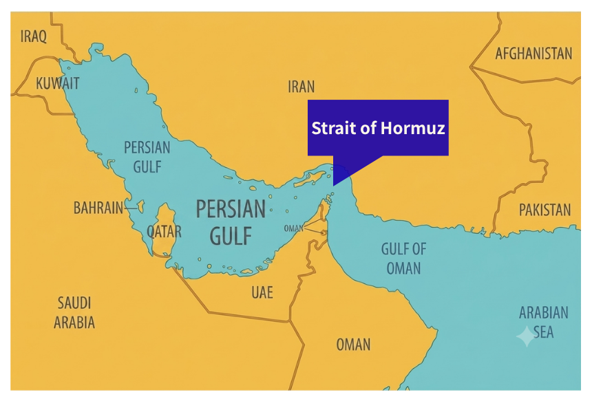
1. The Strait of Hormuz is the waterway through which crude oil and LNG loaded in the Persian Gulf pass to reach the open sea (the Gulf of Oman, the Arabian Sea, and the Indian Ocean), with traffic separated under a Traffic Separation Scheme (TSS) set and administered by the IMO. This function as a navigation channel is what makes the Strait not merely a geographic narrows, but a route operated under an internationally agreed set of rules.
2. For the seven principal Persian Gulf coastal states — Saudi Arabia, the UAE, Kuwait, Qatar, Iraq, Bahrain, and Iran — the Strait is the primary maritime export route, with the bulk of the oil that transits it (roughly 80–90%) bound for Asian markets (China, India, Japan, South Korea, and others).
3. Land routes that avoid the Strait entirely face quantitative limits. Saudi Arabia (the Petroline pipeline) and the UAE (the Abu Dhabi crude pipeline) both have pipelines capable of bypassing the Strait, but their combined available capacity is only around 3.5 to 5.5 million barrels per day — a fraction of the Strait's roughly 20 million bpd total flow.
<Example>
A Very Large Crude Carrier (VLCC, carrying roughly 200,000 to 300,000 tonnes) sails approximately 12,000 km from the Persian Gulf to Japan, a voyage of roughly three weeks one way. Japan depends on the Middle East for 95.9% of its crude oil imports, making this route a lifeline for the country's energy security.
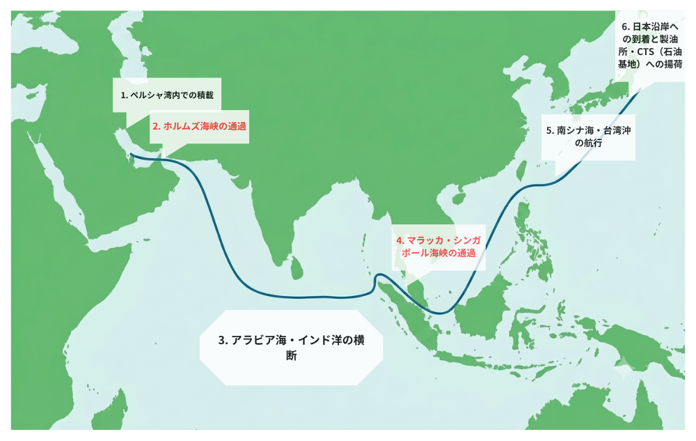
- Main ports: Ras Tanura (Saudi Arabia), Jebel Dhanna (UAE), Mina Al Ahmadi (Kuwait), and others.
- As Japan's Ministry of Economy, Trade and Industry / Agency for Natural Resources and Energy reported (data for March 2026, published April 30, 2026), the VLCC loads roughly 2 million barrels of crude, underpinning the 95.9% Middle East dependency of Japan's oil imports.
- The vessel transits the Strait of Hormuz, the Persian Gulf's sole maritime outlet, passing through into the Gulf of Oman.
- It follows the designated route under the IMO's Traffic Separation Scheme (TSS).
- From the Gulf of Oman the vessel enters the Arabian Sea and heads east across the Indian Ocean, passing south of the Indian subcontinent (off Sri Lanka).
- The vessel transits the narrow Strait of Malacca and Singapore Strait, between Sumatra (Indonesia) and the Malay Peninsula.
- Navigational constraint: a maximum draft limit of roughly 20 metres governs the navigation of deep-draft vessels.
- Clearing the Strait of Malacca, the vessel enters the South China Sea and heads northeast, passing off Taiwan (or through the Bashi Channel) into the Pacific.
- The vessel arrives at one of Japan's major refineries or crude terminals — Kiire, Keihin, Hanshin, Yokkaichi, and others.
- It connects to pipeline infrastructure and discharges the crude into storage tanks.
<Challenges and Caveats>
1. Japan's seaborne supply route runs through two major chokepoints — the Strait of Hormuz and the Strait of Malacca/Singapore. The roughly 20-metre draft limit at Malacca/Singapore can force deep-draft vessels to divert via the Lombok Strait (east of Bali), and the added distance increases voyage time, fuel consumption, and charter costs. The Strait of Hormuz's own bypass capacity (3.5–5.5 million bpd via pipeline) is limited, and Qatari and UAE LNG has no land-based alternative route around the Strait at all.
2. Even short of an actual physical closure, shipping's contractual structures and insurance regime can effectively suspend operations. The Joint War Committee of the London insurance market designates the waters around the Strait of Hormuz as a Listed Area, which can trigger additional war risk premiums. Under standard clauses such as BIMCO's CONWARTIME, owners and masters retain the contractual right to refuse to continue a voyage where war risk is reasonably judged to have increased.
3. Because the voyage from the Middle East takes roughly three weeks, tankers already at sea (floating inventory) continue arriving in sequence even if a loading disruption occurs at origin — meaning physical supply does not halt instantly. Oil prices, freight rates, and insurance costs, however, tend to react to a rise in geopolitical tension well ahead of any actual disruption to arrivals. A clear gap exists between the timeline of physical transport and the timeline priced in by financial markets.
4. Domestic strategic petroleum reserves act as a buffer against supply disruption, but their use is subject to institutional and time-related constraints. Japan holds 210 days' worth of reserves by its domestic standard (179 days under the IEA standard), but the process from releasing reserve oil to refining and domestic distribution takes a meaningful amount of time. It is also worth noting that emergency reserve systems exist to cushion the shock of a physical supply disruption — they are not designed to suppress a rise in market prices itself.
- International Energy Agency, "Strait of Hormuz" (iea.org/about/oil-security-and-emergency-response/strait-of-hormuz) — primary source on transit volume (~20 mb/d, ~25% of world seaborne trade), bypass pipeline capacity (3.5–5.5 mb/d), and the share bound for Asia
- International Energy Agency, "Strait of Hormuz Factsheet" (2026 edition, iea.blob.core.windows.net) — primary source on LNG transit share (~19–20% of world trade) and the export structure of the seven coastal states
- International Maritime Organization, "Ships' Routeing" (imo.org) — primary source on the Traffic Separation Scheme (TSS) established for the Strait of Hormuz
- U.S. Energy Information Administration, "World Oil Transit Chokepoints Analysis" (eia.gov) — primary source on the draft constraint at the Strait of Malacca and on chokepoint analysis
- Japan's Ministry of Economy, Trade and Industry / Agency for Natural Resources and Energy, "Petroleum Statistics Report" (enecho.meti.go.jp) — primary source on Japan's Middle East dependency for crude oil imports (95.9%, March 2026 data)
- Japan's Ministry of Economy, Trade and Industry / Agency for Natural Resources and Energy, "Status of Petroleum Reserves" (published June 2026) — primary source on Japan's reserve days (210 days domestic standard / 179 days IEA standard)
- Baltic and International Maritime Council, "Standard War Risks Clause for Time Charter Parties 2013 (CONWARTIME 2013)" (bimco.org) — primary source on the right to refuse navigation when war risk increases
- Joint War Committee (Lloyd's Market Association), "Hull War, Piracy, Terrorism and Related Perils Listed Areas" (lmalloyds.com) — primary source on the Listed Area designation of waters around the Strait of Hormuz
Strait of Malacca
マラッカ海峡 Geopolitics ✓ Verified Citations Market Practitioner Term<Mechanism>
The Strait of Malacca lies on the maritime route linking the Indian Ocean side to East and Southeast Asia, and is used by vessels carrying crude oil, petroleum products, and LNG from resource-supplying regions such as the Middle East and Africa to demand centers including China, Japan, and South Korea. It therefore functions as a maritime channel connecting the regions that produce and load resources with the Asian markets that consume them. The IMO likewise positions the Strait of Malacca as a principal shipping route between the Indian Ocean and the Pacific.
Resources loaded onto vessels in supplier regions cross the Indian Ocean, pass through the Strait of Malacca, and are transported via the South China Sea and other waters to demand centers in East Asia. Maritime transport through the Strait is therefore not confined to a single commodity or a single country's trade, but forms part of an international logistics network linking multiple supplier and consumer countries. The EIA likewise positions the Strait of Malacca as a principal sea route linking Middle Eastern oil and natural gas suppliers with markets in East and Southeast Asia.
As multiple supply and demand regions are connected in this way by maritime transport, large volumes of vessels and cargo flow continuously into the Strait of Malacca. As a result, the Strait becomes not merely a "place of passage" but an important node through which international logistics, including energy, continuously flow. The IMO indeed treats the Malacca and Singapore Straits as an international shipping route with particularly heavy traffic, and a framework has been built in which coastal states, user states, and the shipping industry jointly manage the waterway for navigational safety.
Because large numbers of vessels continuously navigate the same waters, there is a need to maintain safe passage while preventing collisions, groundings, and environmental pollution. Accordingly, a cooperative framework has formed centered on the coastal states of Indonesia, Malaysia, and Singapore, with user states and shipping-industry stakeholders also participating. In 2007, the Cooperative Mechanism was launched with IMO support, building a framework for cooperation on navigational safety, environmental protection, and the maintenance of aids to navigation.
As a result, vessels carrying cargo from resource-supplying regions to demand regions in Asia continuously pass through the Strait of Malacca, combined with the route management and international cooperation needed to sustain that navigation. The Strait of Malacca thus functions not merely as a geographic strait, but as transport infrastructure that actually connects Asia's energy markets with international seaborne trade.[1][2][3][6][8]
<Examples>
- Much of the crude oil and LNG loaded in the Persian Gulf in the Middle East (i.e., cargo that has already passed through the Strait of Hormuz) crosses the Indian Ocean and then exits through this Strait toward the South China Sea and the Pacific side (China, Japan, South Korea, and others).
- In this sense, the Strait of Malacca sits as the second stage of a "dual chokepoint arranged in series" alongside the Strait of Hormuz, forming the final leg of the energy transport route for major Asian economies with high dependence on the Middle East.
- The Strait is roughly 233km wide at its northwestern end (between Sumatra and the Malay Peninsula), but narrows sharply toward the southeast.
- Off Singapore, at the Phillips Channel, the navigable width converges to about 2.8km — this narrowest point is the bottleneck that effectively governs the Strait's overall navigational capacity.
- Shoals exist along the route, and depths near One Fathom Bank and similar areas are only around 23m.
- Given this depth constraint and the required under-keel clearance (UKC), the largest vessel type able to transit the Strait fully laden — with a draft of about 20.5m — is referred to in practice as "Malaccamax," with VLCCs of roughly 300,000 DWT as the representative vessel type. Larger-draft vessels beyond this use alternative routes such as the Lombok or Sunda Straits, depending on route conditions.
- The Traffic Separation Scheme (TSS) established under the IMO is jointly operated by the Tripartite Technical Experts Group (TTEG), comprising Indonesia, Malaysia, and Singapore.
- Vessels of 300 gross tons and above are subject to a mandatory ship reporting system (STRAITREP), under which they must report their position and movements to the coastal states' Vessel Traffic Service (VTS); use of pilotage is also recommended for deep-draft vessels. These systems allow the large volume of high-density vessel traffic in this narrow waterway to proceed in an orderly manner.
[1][2][6][7][9][10][11][12]
<Challenges and Considerations> The Strait of Malacca currently carries about 29% of the world's seaborne oil transport (roughly 23.2 million barrels per day, EIA, 2026) and about a quarter of maritime trade overall passes through it (World Ocean Review, 2017). Its geographic structure — roughly 800km in length and about 50km at its narrowest — has, over centuries, given coastal states locational advantages (geographic rent) through transit and port services. Will this advantage remain fixed going forward?
A factor that could unsettle this premise is the retreat of Arctic sea ice due to global warming and the resulting expansion of the commercial viability of the Northern Sea Route (NSR/Northeast Passage). In 2014, in testimony before the UK House of Lords Select Committee on the Arctic, Japan's Ambassador to the UK stated that a viable Northern Sea Route could cut the distance between Japan and major European ports (such as Hamburg and Rotterdam) by as much as around 40%, and stated explicitly that a motivation was to diversify transport away from dependence on the Strait of Malacca, the Indian Ocean, and the Philippine sea lanes (House of Lords, 2015). Singapore's High Commissioner to the UK, also present, testified that Singapore had decided to join the Arctic Council on the understanding that this structural shift was "not a short-term but a medium-term matter" — consistent with the fact that Singapore obtained observer status on the Council in 2013 (Singapore MFA, 2013).
China has further formalized this trend as national strategy: in its 2018 "China's Arctic Policy" white paper, it set out the development of the Northern Sea Route and the building of a "Polar Silk Road" with other countries as official policy (State Council Information Office of China, 2018). China Ocean Shipping Company (COSCO) conducted a trial shipment of wind-power components from Tianjin to three European countries via the Northern Sea Route in 2016, and in the same year a Chinese company acquired a 12.5% stake in a Greenland resource company, among other moves positioning China on both the resource and infrastructure fronts. Plans are also proceeding to develop Hunchun, near the China–Russia border, as a future logistics hub, in a move reportedly aimed at becoming a "northern hub" comparable to Singapore (World Ocean Review, 2017).
That said, it is unlikely that the Northern Sea Route will substitute for the Strait of Malacca in the short term. Academic research points out that the ice-free navigation window remains limited over the course of a year, with ice conditions constraining navigation for extended periods (Idris & Ramli, 2018). It has also been quantitatively shown that expanded NSR use carries its own cost in the form of increased emissions, with estimates suggesting the resulting climate feedback cost could offset roughly 25–33% of the economic benefit from shorter transport distances (Yumashev et al., 2017). The Northern Sea Route should therefore be understood not as an "immediate substitute for the Strait of Malacca," but as a factor that could, over the long term, diversify logistics structures and relativize the Strait's geographic advantage.
Singapore has been the quickest to sense this structural shift and act on it. The country had only a single public research institute as of 1987, but has since expanded R&D investment and now hosts more than twenty such institutions. Between 2003 and 2006 it built the Biopolis life-sciences research hub, among other steps advancing a shift from an economic model dependent on "geographic port location" toward a knowledge-intensive model dependent on "homegrown intellectual property and technology" (World Ocean Review, 2017). Malaysia and Indonesia have likewise pursued industrial foundations that go beyond being mere transit points, through the development of Penang's special economic zone and the expansion of the Medan metropolitan area on Sumatra (World Ocean Review, 2017). For Indonesia in particular, recent empirical research points out that factors such as logistics integration, institutional efficiency, and port digitalization — rather than geographic advantage as a coastal state per se — are increasingly the main determinants of maritime competitiveness (JISS, 2026).
The essential question surrounding the Strait of Malacca is therefore not the simple question of substitutability — "when will the Northern Sea Route replace the Strait of Malacca." Rather, it comes down to the capacity of the coastal states themselves to transform their structures: given the irreversible external shift posed by climate change and major powers' Arctic strategies, which risks eroding the "absoluteness of geographic location" over the long term, how quickly can these states — Singapore above all, a small country with few resources beyond its geographic advantage — sense this risk and transform their port and logistics functions from a "location-dependent" model into a sustainable, "technology-, institution-, and network-integrated" hub.[1][13][14][15][16][17][18][19]
- [1] U.S. Energy Information Administration (EIA), 2026, "World Oil Transit Chokepoints"
- [2] International Maritime Organization (IMO), "Safety of straits used for international navigation — FAQs"
- [3] IMO (2015), "Safety and sustainability in Straits of Malacca and Singapore"
- [4] IMO, "Singapore Maritime Lecture"
- [5] IMO, "Seminar on CSR activities for the shipping industry" (an older source, used only to support the historical significance of vessel-count and trade-share figures)
- [6] Singapore Maritime and Port Authority (MPA), "Vessel Traffic Information System"
- [7] Singapore MPA, "Voluntary Pilotage Services in the Straits of Malacca and Singapore"
- [8] EIA (2018), "More than 30% of global maritime crude oil trade moves through the South China Sea"
- [9] JICA, "Joint Hydrographic Survey in Malacca and Singapore Straits"
- [10] Nippon Foundation, "The Situation in the Malacca and Singapore Straits"
- [11] Qu, X. & Meng, Q. (2012), "The economic importance of the Straits of Malacca and Singapore: An extreme-scenario analysis," Transportation Research Part E: Logistics and Transportation Review 48(1), 258–265
- [12] Navigational regulation materials produced by the NUS Centre for International Law
- [13] maribus gGmbH (2017), "World Ocean Review 5: Living with the Coasts — The Strait of Malacca: a historical shipping metropolis"
- [14] House of Lords, Select Committee on the Arctic, Evidence Session No.24 (testimony of 25 November 2014, included in the 2015 report "Responding to a Changing Arctic")
- [15] Singapore Ministry of Foreign Affairs (2013), "Press Statement: Singapore granted observership in the Arctic Council"
- [16] State Council Information Office of China (2018), "China's Arctic Policy"
- [17] Yumashev, D., van Hussen, K., Gille, J., & Whiteman, G. (2017), "Towards a balanced view of Arctic shipping," Climatic Change 143, 143–155
- [18] Idris, H. & Ramli, M. F. (2018), "Southeast Asian Region Maritime Connectivity and the Potential Development of the Northern Sea Route for Commercial Shipping," JATI 23(2), 25–46
- [19] Langelo, F. N. & Aprilia, C. (2026), "Maritime Logistics, Geo-Economic Integration, and Economic Rent Capture in the Malacca Strait," JISS 7(6)
Chokepoints
チョーク・ポイント Geopolitics ✓ Verified Citations Market Practitioner Term<Mechanism> The world's maritime trade network is structurally dependent on specific nodes — natural chokepoints (straits) and man-made ones (canals). These points face physical capacity constraints, and when their transit function is disrupted by accidents, natural disasters, geopolitical tension, military blockades, or piracy, international logistics can be severely interrupted. Disruption at a chokepoint structurally pushes up global logistics costs and supply-chain-wide risk premium, through longer shipping distances (rerouting), vessel demurrage, higher fuel consumption from longer voyages, and surging freight rates and marine insurance premiums.
<Example> International organizations such as the United Nations Conference on Trade and Development (UNCTAD) and the International Maritime Organization (IMO) identify a set of major global chokepoints, including the Strait of Hormuz, the Strait of Malacca, the Suez Canal, the Bab-el-Mandeb Strait, the Panama Canal, the Turkish Straits, and the Danish Straits. For example, official reports have documented large-scale vessel congestion at the Suez and Panama Canals caused by major vessel groundings and drought-driven draft and transit restrictions, substantially delaying container ships, bulk carriers, and various tankers worldwide. Similarly, a deteriorating security environment around the Bab-el-Mandeb Strait — the passage from the Red Sea to the Gulf of Aden — has led commercial shipping to reroute via the Cape of Good Hope, substantially lengthening transit times between Europe and Asia and reducing effective global shipping capacity while raising freight rates (UNCTAD, 2024).
<Issues and Caveats>
1. Limits on physical substitution capacity — Even where alternative infrastructure exists, such as overland pipelines, land transport networks, or bypass routes, their capacity is often limited relative to total throughput of the strait or canal itself, and in many cases cannot fully substitute for a large-scale disruption.
2. Risk of compounded concentration — Chokepoints are not isolated bottlenecks; several major routes can form a chained structure (for example, sequential transit through the Suez Canal and the Bab-el-Mandeb Strait), meaning a localized regional risk can propagate across the entire global trade network.
3. Structural cost effects — Higher defensive escort costs, the application of war-risk insurance premiums, and increased working-capital costs from longer transit times can all feed through into final commodity price formation.
- UNCTAD (2024) "Review of Maritime Transport 2024: Navigating Maritime Chokepoints," United Nations Conference on Trade and Development — Primary source analyzing transit disruption at major global chokepoints and its impact on logistics costs
- International Maritime Organization (IMO) "Reports on Acts of Piracy and Armed Robbery Against Ships," MSC.4/Circ. series — Primary source publishing monthly data on piracy and armed robbery incidents around chokepoints
Cape of Good Hope
喜望峰 Geopolitics ✓ Verified Citations Market Practitioner Term<Mechanism>
① Multiple routes can connect the same origin and destination in international maritime transport
For maritime transport linking Europe with Asia and the Middle East, the route passing through the Suez Canal, the Red Sea, and the Bab-el-Mandeb Strait serves as the main short-distance route. At the same time, a route around the southern tip of Africa via the Cape of Good Hope also exists. In other words, the Cape of Good Hope is not a point where cargo concentrates at a particular strait, but a point offering a separate maritime route from the existing main routes. It is positioned as a "major trade route and alternative route."
② When a constraint arises on the main route, vessels switch routes themselves
The Suez Canal and the Bab-el-Mandeb Strait are important routes connecting Europe and Asia over a short distance. Accordingly, when security concerns, route blockages, or similar issues make them difficult to use, vessels can avoid passing through that route altogether. Vessels avoiding the Bab-el-Mandeb Strait have indeed been observed switching to a route via the Cape of Good Hope around the southern tip of Africa.
③ The Cape of Good Hope becomes an alternative route that absorbs that cargo and those vessels
When a route shifts from the Suez/Red Sea route to the Cape of Good Hope route, the cargo itself does not stop; the same supply and demand regions can instead be connected via a different maritime route. This is the essence of the Cape of Good Hope, which is explicitly described as an "alternative sea route" that bypasses the Gulf of Aden, the Bab-el-Mandeb Strait, and the Suez Canal.
④ As a result, international logistics "connectivity" is maintained
Because the Cape of Good Hope exists as an alternative route, vessels can still transport cargo to its destination via another route even when the main route is unavailable. UNCTAD likewise shows that, amid disruption in the Red Sea, vessels rerouted via the Cape of Good Hope, which kept the flow of global freight moving while increasing distance, time, and cost.
⑤ "Being able to substitute" and "the cost of substituting" occur together
Because the Cape of Good Hope can physically substitute for the main route, it has the function of averting a stoppage in international logistics. At the same time, because the route is longer than via Suez, vessels that switch incur additional sailing time, fuel, and vessel tie-up. For transport from the Arabian Sea to Europe, the Cape route can take around 15 days longer than the Suez route.
⑥ The mechanism of the Cape of Good Hope therefore lies in "route substitutability," and the use of that alternative route can affect the market
Main route available → Suez/Red Sea route used ↓ Constraint on main route → route avoided ↓ Cape of Good Hope alternative route available → vessel/cargo flow shifts to the Cape ↓ International logistics connectivity maintained → transport to supply and demand regions continues ↓ In exchange, sailing distance, time, and transport cost increase → impact on vessel demand, fleet supply-demand, freight rates, and other market factors
In other words, the essence of the Cape of Good Hope is not that it concentrates or halts traffic the way a chokepoint does, but that when a constraint arises on the use of a chokepoint or similar route, it functions as an "alternative route" that shifts the flow of international maritime transport to another path and maintains the connection between supply and demand regions. The use of that alternative route can in turn change sailing distance, time, and transport cost, which can also affect the shipping market.[1][2][5]
<Examples> The 2023 Red Sea disruption
From late 2023, following attacks on merchant vessels by Yemen's Houthi movement, shipping companies avoided the Bab-el-Mandeb Strait and the Red Sea and switched to a route via the Cape of Good Hope at the southern tip of Africa.
- Following attacks on vessels around the Red Sea in late 2023, many merchant shipping operators chose routes avoiding the Bab-el-Mandeb Strait and the Red Sea.
- Indeed, in December 2023 the volume of crude oil transiting the Bab-el-Mandeb Strait fell by about 18% from the January–November 2023 average, and the volume of petroleum products fell by about 30% compared with the rest of 2023.
- Vessels avoiding the main route switched to a route around the southern tip of Africa via the Cape of Good Hope. As a result, the volume of crude oil and petroleum products transiting around the Cape of Good Hope rose from a 2023 average of 5.9 million b/d to 8.7 million b/d in January–May 2024, an increase of about 47%.
- This increase is also reflected in actual trade flows. Crude oil producers in Saudi Arabia and Iraq began shipping more crude to Europe around the Cape rather than via the Suez Canal. Refiners in Asia and the Middle East likewise redirected petroleum products bound for Europe via the Cape.
- As a result, volumes around the Cape of Good Hope itself rose substantially. 2023 average: 5.9 million b/d; January–May 2024: 8.7 million b/d; increase: about 2.8 million b/d; growth rate: about 47%.
- In addition, US oil trade around the Cape of Good Hope rose by about a third, or just over 600,000 b/d, in January–May 2024 versus the 2023 average. Crude oil and petroleum product volumes moving from Russia to Asia via the Cape were also nearly four times the full-year 2023 level in January–May 2024.
- In other words, as use of the Red Sea and Bab-el-Mandeb Strait declined, volumes moving via the Cape of Good Hope increased.
- This is a case in which the "alternative route" mechanism described in ② — a constraint on the use of the Red Sea/Bab-el-Mandeb Strait leading vessels to avoid the main route, reroute via the Cape of Good Hope, and increase actual cargo flow around the Cape — was confirmed in actual maritime transport data.
- While transport itself continued after the shift to the Cape route, the route became longer. For transport from the Arabian Sea to Europe, the Cape route is said to take around 15 days longer than via the Bab-el-Mandeb Strait and Suez Canal, adding to transport cost and time.
- UNCTAD has also confirmed that vessel capacity arriving via the Cape of Good Hope rose by 89% in 2024, and that while this rerouting kept cargo flows moving, it also raised costs through greater distance and time. It further estimates that rerouting away from the Red Sea and the Panama Canal pushed up global vessel demand by 3% and container ship demand by 12% by mid-2024.
- Geopolitical shock → reduced use of the Bab-el-Mandeb Strait and Red Sea → vessels avoid the main route → reroute via the Cape of Good Hope → crude oil and petroleum product flows around the Cape rise from 5.9 million b/d to 8.7 million b/d → the actual seaborne transport route is displaced → transport connectivity to Europe, Asia and elsewhere is maintained → sailing distance, time, and cost increase → potential impact on vessel demand and other market factors.
- This Red Sea disruption from late 2023 onward is a case in which the Cape of Good Hope's function as an "alternative route" — a constraint on the use of a chokepoint leading vessels to reroute via the Cape and actual cargo flows to shift there — is confirmed by real transport data.
[2][3][6]
<Challenges and Considerations> How an alternative route changes a chokepoint's geopolitical leverage
A chokepoint's geopolitical importance is not determined solely by the volume of traffic that passes through it. Its influence also depends on how much international maritime transport can shift to another route when that point becomes unusable.
For the Suez Canal and the Bab-el-Mandeb Strait, the Red Sea disruption from late 2023 onward triggered a large-scale, real-world shift in routing. According to UNCTAD, as of June 2024, compared with the mid-December 2023 average, vessel transport capacity through the Suez Canal had fallen 70%, capacity around the Bab-el-Mandeb Strait had fallen 76%, while vessel transport capacity arriving via the Cape of Good Hope had risen 89%.[2]
OECD analysis further shows that, by the end of the first quarter of 2024, trade volume around the southern tip of Africa had risen to about four times that via Suez, while total traffic across both routes combined showed little change. This demonstrates, using actual trade flow data, that when a constraint arises on the use of a chokepoint, international maritime transport does not simply stop; traffic can instead be reallocated to another route within the network.[7]
This point matters for thinking about a chokepoint's "scarcity." A relationship can hold in which a constraint on a chokepoint leads to rerouting via the Cape of Good Hope, cargo and vessel transport itself continues, and the chokepoint's power to "physically halt logistics" is relativized as a result.
Indeed, a 2025 study published in Nature Communications estimates the systemic risk of 24 global maritime chokepoints, explicitly distinguishing between the presence of alternative routes and the rerouting distance involved. The Suez Canal and the Bab-el-Mandeb Strait are classified as chokepoints requiring long-distance rerouting of over 5,000km; the study shows that at both points, the trade impact of geopolitical risk is large, and that even where an alternative route exists, using it can carry substantial economic loss.[8]
The same study estimates the expected value of global trade disrupted annually by chokepoint disruptions at about USD192 billion. It further estimates annual economic losses from delays, rerouting, insurance premiums, and trade disruption at USD10.7 billion, and the impact on freight rates from reduced fleet capacity due to rerouting at an additional USD3.4 billion per year. The Suez Canal and the Bab-el-Mandeb Strait are major sources of this economic risk.[8]
In other words, "an alternative route existing" is not synonymous with "a chokepoint's strategic importance disappearing." Rather, what can be confirmed from ①–③ above is a more complex structure: a constraint on a chokepoint's use → rerouting via the Cape of Good Hope → logistics network connectivity is maintained → but sailing distance and time increase → additional burden on vessel tie-up time, required fleet capacity, fuel, insurance, freight rates, and the like → the chokepoint's constraint spills over as a burden on the global maritime transport network as a whole.
UNCTAD shows that, for the Shenzhen–Rotterdam route, the Suez route runs about 10,000 nautical miles and 31 days, versus about 13,000 nautical miles and 41 days via the Cape of Good Hope. It also estimates that rerouting via the Cape pushed up global vessel demand by about 3% and container ship demand by about 12%.[2]
The EIA likewise positions the Cape of Good Hope not as a chokepoint itself, but as an alternative maritime route bypassing the Suez Canal, the Bab-el-Mandeb Strait, and similar points. For voyages from the Arabian Sea to Europe, the Cape route can add around 15 days of additional sailing time.[1]
The important conclusion that follows is that a chokepoint's geopolitical leverage cannot be evaluated solely by its "ability to halt logistics." Where an alternative route such as the Cape of Good Hope exists, a constraint on access to a chokepoint does not necessarily bring global logistics to a complete stop. Instead, by forcing a detour, it places an additional burden on international maritime transport as a whole, through distance, time, vessel demand, transport cost, and network congestion, among other channels.
The existence of the Cape of Good Hope therefore cannot simply be said to "weaken" a chokepoint's geopolitical leverage. Rather, it can change how that leverage manifests — from "the power to directly cut off logistics" to "the power to force rerouting via an alternative route and place additional burden on the logistics network."
It is important to note here that this "change in leverage" is not a fact directly quantified by primary sources, but an analytical implication drawn from empirical results concerning actual rerouting, trade flows, vessel demand, transport time and distance, and economic losses. What the primary sources confirm is the fact that, in response to a constraint on chokepoint use, large-scale rerouting to the Cape of Good Hope actually occurred, that this kept logistics connected, while placing an additional burden on the global maritime transport network.
In short, the essential challenge posed by the Cape of Good Hope is not only "whether it can economically substitute for the Suez Canal." It also concerns how the existence of this alternative route changes a chokepoint's geopolitical scarcity and leverage, and how that effect propagates from an individual route to the global maritime transport network as a whole.
- [1] U.S. Energy Information Administration (EIA), "World Oil Transit Chokepoints"
- [2] UNCTAD, Review of Maritime Transport 2024
- [3] EIA, "Red Sea disruptions increase oil flows around Cape of Good Hope" (2024)
- [4] UNCTAD, Review of Maritime Transport 2025
- [5] UNCTAD, "Suez and Panama Canal disruptions threaten global trade and development"
- [6] EIA, "Red Sea attacks increase shipping times and freight rates" (2024)
- [7] OECD (2024), Risks and Resilience in Global Trade: Key Trends in 2023-2024, OECD Publishing, Paris
- [8] Verschuur, J., Lumma, J. & Hall, J.W. (2025), "Systemic impacts of disruptions at maritime chokepoints," Nature Communications 16, 10421
Suez Canal
スエズ運河 Geopolitics ✓ Verified Citations Market Practitioner Term<Mechanism>
① Directly connecting the Mediterranean and Red Sea shortens maritime transport between different sea areas
When connecting Europe and the Mediterranean region with Asia and the Indian Ocean region by sea, transiting the Suez Canal removes the need to round the southern tip of Africa. The Suez Canal Authority (SCA) positions the Suez Canal as the shortest maritime route linking east and west, stating that, compared with the Cape of Good Hope route, it can reduce sailing distance, time, fuel consumption, and vessel operating costs.
② As the route shortens, vessels transit the Suez Canal
Because the Suez Canal shortens sailing distance and sailing time, vessels connecting Europe and Asia have an economic incentive to choose the route via the Suez Canal. The SCA indeed cites the canal's shortest, fastest route — a function of its geographic position — as the reason modern vessels make extensive use of it.
③ As a result, the Suez Canal functions as a connecting point linking different sea areas and regions
Transiting the Suez Canal allows maritime transport to continue seamlessly from the Mediterranean to the Red Sea and on to the Indian Ocean. In other words, Suez's function is not simply that vessels "pass through the canal," but that it links maritime transport between different sea areas and regions through a single connecting point. The SCA likewise positions Suez as a key international route linking the Mediterranean and the Red Sea.
④ This connecting function is built into the global maritime transport network
As numerous routes linking Europe and the Mediterranean region with Asia and the Indian Ocean region pass through Suez, the Suez Canal becomes a node in the network connecting maritime transport between different regions, beyond the individual sailing routes of any one vessel.
⑤ The mechanism of Suez therefore lies in its "function as a connecting node"
Directly connects the Mediterranean and Red Sea → shortens the Europe-Asia route → vessels choose to transit Suez → connects transport across different sea areas and regions → Suez functions as a node in the international shipping network
In other words, the essential mechanism of Suez is that it directly connects geographically separated sea areas, thereby shortening routes, and as a result concentrates and connects maritime transport between different regions at a single connecting point.[1][2]
<Examples> Asia–Europe liner services, 2026 — actual Asia–Europe shipping services transiting the Suez Canal
- Because the Suez Canal crosses the Isthmus of Suez to directly connect the Mediterranean and the Red Sea, it can link Mediterranean-side European ports with Asian ports reached via the Red Sea and Indian Ocean as a single maritime route. For Europe-Asia maritime transport, a route forms that connects the two regions via the Suez Canal without a large detour around the southern tip of Africa.
- The SCA likewise positions the Suez Canal as the shortest maritime transport route linking Europe with the Indian Ocean and western Pacific region.
- Along the formed route, regular shipping services linking Europe and Asia actually operate. For example, the SCA recorded that in June 2026, the container ship CMA CGM VENDOME, bound from France to Malaysia, transited the Suez Canal.
- The vessel operates as part of a shipping service connecting the Far East and North-West Europe, and a single continuous voyage via the Suez Canal, from a European port to an Asian port, actually took place.
- As a vessel bound from France to Malaysia transits the Suez Canal, the Mediterranean, the Red Sea, and the Indian Ocean — different sea areas — are linked into a single continuous voyage, and actual cargo transport takes place between European and Asian ports.
- The SCA also recorded, in August 2026, the container ship BANGKOK MAERSK, bound from Italy to Singapore, transiting the Suez Canal. This vessel too is built into a shipping service connecting Europe and Asia; the Suez Canal is not simply a waterway that vessels pass through, but functions as a point that actually connects European and Asian ports through real shipping services.
- Because the Suez Canal directly connects the Mediterranean and the Red Sea, seaborne transport from Europe to Asia is established as a single continuous route, and actual vessels use that route.
- This actual voyage activity is a case in which the mechanism shown in ② — directly connecting the Mediterranean and Red Sea → forming a Europe-Asia route → vessels choosing to transit Suez → connecting transport across different sea areas and regions → Suez functioning as a node in the international shipping network — appears as an actual shipping flow.
- Behind this connection's actual use in shipping is the fact that transiting Suez shortens route distance and transport time. The SCA explains that, for an actual voyage from Shanghai to Turkey, the Cape of Good Hope route runs about 14,600 nautical miles versus about 8,071 nautical miles via the Suez Canal — a distance reduction of about 45%.
- By directly connecting the Mediterranean and Red Sea and shortening Europe-Asia maritime transport, the Suez Canal draws actual vessels and cargo to this connecting point, forming a structure that is continuously used within the international shipping network.
- Directly connecting the Mediterranean and Red Sea → forming a Europe-Asia maritime route → actual vessels using that route → transport flows established between European and Asian ports → the Suez Canal functioning as a connecting node in the international shipping network. The actual Asia–Europe shipping services recorded by the SCA in 2026 concretely demonstrate this causal chain.
- The essence of this case, then, is not simply "a ship passed through the Suez Canal," but that the Suez Canal's direct connection of the Mediterranean and Red Sea establishes actual Europe-Asia maritime transport and builds that transport into the international shipping network.[1][4][5][6]
<Challenges and Considerations> How dependence on a single connecting node affects the maritime transport network
In considering the Suez Canal's geopolitical importance, what matters is not the volume of cargo passing through the canal alone. Built within Egyptian territory, the Suez Canal connects the Mediterranean and the Red Sea, functioning as a node in maritime transport linking Europe and the Mediterranean region with Asia and the Indian Ocean region. The Suez Canal Authority (SCA) itself positions the canal as a maritime trade route supporting "the safe and sustainable flow of world trade." (SCA)[1]
The challenge arising from this structure is that dependence on a single connecting point can affect the connectivity of the entire maritime transport network, beyond the problems of any individual route.
Feyrer's natural experiment (an analytical method that treats an external event as if it were an experiment, to test a causal relationship), using the canal's 1967 closure and 1975 reopening, confirms that bilateral trade changed significantly as a result of an exogenous change in sea distance caused by the canal's closure. The study uses the distance shock from the Suez closure to isolate the effect of transport distance and cost itself more clearly than conventional international trade analysis, showing that an increase in sea distance reduces trade. It also shows that the adjustment in trade volume takes time, with roughly three years elapsing after the shock before adjustment is complete. (Feyrer, 2021)[13]
This result shows that a stoppage in Suez's function is not merely a localized phenomenon of "a ship taking a different route," but can change the economic conditions of connectivity between regions themselves.
A further study analyzing the global shipping network using AIS data (Automatic Identification System data — position and navigation data broadcast by vessels) examined the 2021 Ever Given blockage, comparing the Suez blockage with a random network disruption of similar scale; it found that the Suez blockage had a greater impact on the network's accessibility and connectivity. The impact varies by region, with the effect on African port networks found to be particularly large. (Wan et al., 2023)[14]
What emerges here is that Suez's importance cannot be explained solely by "how much traffic passes through it." Because Suez handles connectivity between different regions within the global shipping network, a disruption at this one node can spill over not only to vessels directly using it, but to other ports, routes, and fleet deployment as well.
A 2025 study by Verschuur, Lumma and Hall generalizes this point further. The study integrates country-level trade dependency, the shipping network, and the natural and man-made hazards that could occur at each chokepoint, to quantify the systemic impact of chokepoint disruptions across 24 maritime chokepoints. For the Suez Canal, it estimates that about 15% of global maritime trade value passes through it, and estimates the Expected Value of Trade Disrupted (EVTD — an annual expected value, weighted by probability, of the trade value exposed to disruption risk from a chokepoint disruption; not an amount of loss that has actually occurred) from disruption at USD44.2 billion per year. It further identifies the Suez Canal as a major contributor to economic risk from delay, rerouting, insurance premiums, and trade disruption. (Verschuur et al., 2025)[15]
One further finding of the same study is that, because a single trade flow can pass through multiple chokepoints, the impact of chokepoints is not an independent, point-level risk but can overlap across the network. The study estimates that, aggregating trade flows through the 24 chokepoints, an average of USD1.80 of trade passes through a chokepoint for every USD1 of seaborne trade. (Verschuur et al., 2025)[15]
A consideration for Suez, therefore, is not only "how many vessels could shift to another route if Suez stopped." It also matters which inter-regional connections depend on Suez, and how that dependence overlaps with dependence on other chokepoints.
The Red Sea situation from late 2023 onward provides supporting evidence for this structure. According to UNCTAD, as of June 2024 the gross tonnage of vessels transiting the Suez Canal had fallen by about 70% from the mid-December 2023 level, while vessel capacity arriving via the Cape of Good Hope rose 89%. OECD analysis likewise found that, by the end of the first quarter of 2024, trade volume around the southern tip of Africa had risen to about four times that via Suez, while total traffic across both routes combined showed little change — indicating that the shipping network can reallocate routes in response to a disruption. (UNCTAD, 2024)[10]
The point that follows from this evidence is that dependence on Suez existing is not the same as a stoppage of Suez's function halting world trade. The network has an adaptive capacity for rerouting. At the same time, the fact that rerouting is possible does not mean that structural dependence on Suez disappears. As shown by the 2021 AIS analysis (Wan et al., 2023)[14], the 1967–1975 natural experiment (Feyrer, 2021)[13], and the 2025 systemic-risk analysis (Verschuur et al., 2025)[15], a disruption at a connecting point can affect areas beyond that point itself, through sea distance, network connectivity, trade flows, and fleet deployment.
The core of assessing Suez's geopolitical risk therefore lies not in "the trade volume passing through Suez," but in "how much the network depends on Suez as a single connecting point."
In other words, whereas the problem of a chokepoint arises from "traffic concentrating at a specific point," at Suez that concentration appears as dependence on a connecting function that links different sea areas and regions. The greater this dependence, the more a local disruption can drive a reconfiguration of the shipping network as a whole, with its effects spilling over beyond that point to other regions.
The issue with Suez is not the alternative route itself, but the network structure whereby global seaborne trade's dependence on a single connecting point means that a change in that point's function can spill over into the connectivity and trade flows of the maritime transport network as a whole.
- [1] Suez Canal Authority — About Suez Canal
- [2] Suez Canal Authority — Why Suez Canal? / Importance & Advantages
- [3] Suez Canal Authority — Canal Characteristics
- [4] Suez Canal Authority — AICC HUANGHU transit (13 February 2025)
- [5] Suez Canal Authority — BANGKOK MAERSK (22 August 2026)
- [6] Suez Canal Authority — CMA CGM VENDOME (9 June 2026)
- [7] Suez Canal Authority — Canal History
- [8] Suez Canal Authority — SCA Overview
- [9] Suez Canal Authority — Vision & Mission
- [10] UNCTAD, Review of Maritime Transport 2024
- [11] UNCTAD, Review of Maritime Transport 2025
- [12] OECD, Maritime transportation disruptions and international trade
- [13] Feyrer, J. (2021), "Distance, trade, and income — The 1967 to 1975 closing of the Suez canal as a natural experiment," Journal of Development Economics 153, 102708
- [14] Wan, Z. et al. (2023), "Analysis of the impact of Suez Canal blockage on the global shipping network," Ocean & Coastal Management 245, 106868
- [15] Verschuur, J., Lumma, J. & Hall, J.W. (2025), "Systemic impacts of disruptions at maritime chokepoints," Nature Communications 16, 10421
OVX
原油ボラティリティ指数 GeopoliticsSanctions
制裁 GeopoliticsLiquidation / Cash-out
キャッシュ化(ポジションの現金化) Capital FlowFlight to Cash
キャッシュ化 Capital FlowSquare
スクエア Trading & PositioningSafe-haven Shift
安全資産シフト Capital FlowRotation
ローテーション Capital FlowBalance Sheet Constraint
バランスシート制約 Capital FlowDruzhba Pipeline
ドルジバ・パイプライン GeopoliticsGeopolitical Risk Fatigue
地政学リスク慣れ GeopoliticsStop-loss Cascade
損切り連鎖 Capital FlowProspect Theory
プロスペクト理論 Behavioral Finance ✓ Verified Citations Academic Origin<Mechanism>
At the center of prospect theory is a graph called the "value function," which plots subjective value on the vertical axis against the objective amount of gain or loss on the horizontal axis, tracing an S-shaped curve around a reference point.
On the gain side (to the right), the curve rises, but the additional pleasure from each extra amount grows smaller as the total gets larger — winning $20,000 does not feel exactly twice as good as winning $10,000. The loss side (to the left) behaves the same way, with the feeling change growing smaller as losses accumulate, but the initial drop from the reference point is much steeper than the rise on the gain side. This difference in steepness is what gives "loss aversion" its shape: losing a given amount is felt more strongly than gaining the same amount. Later research puts this difference at roughly a factor of two.
Three properties follow from the shape of this value function. First, reference dependence: what counts as the baseline for evaluation shifts with a person's circumstances (their current holdings, a recent price level), so the same outcome can register as a "gain" or a "loss" depending on where that baseline is set. Second, loss aversion: because of the asymmetric shape described above, people tend to favor safer choices when they are ahead and take on more risk when they are behind — an apparent reversal of ordinary risk attitudes. Third, distortion in how probabilities are felt: people do not weight objective probabilities at face value, instead overweighting low probabilities and underweighting moderate-to-high ones. These three properties were later refined by treating the probability weighting as building up according to the rank of outcomes. [1][2]
<Example> A frequently cited example of prospect theory applied to investor behavior is the "disposition effect" — the tendency to sell a position that shows a gain too quickly, while holding on to a position that shows a loss.
The study that first coined this term did not collect large-scale new data; instead, it reread an existing dataset on individual investors' realized gains and losses through a new theoretical lens. That dataset showed that, of the gains and losses investors chose to realize, roughly 60% were gains and 40% were losses. But a tax-conscious, rational investor would be expected to realize losses more readily, to offset taxable gains, while deferring the realization of gains as long as possible. The observed ratio does not match that tax-rational pattern. Rather than blaming taxes alone for the mismatch, the study explained it by placing loss aversion within a broader framework built from four elements: mental accounting (tracking each position's gains and losses as if it were its own separate account), regret aversion, a struggle with self-control, and tax considerations.
This tendency was confirmed directly in large-scale trading records. An analysis of 10,000 brokerage accounts from 1987 to 1993 found that the rate at which investors realized gains was about 1.5 times the rate at which they realized losses — gains were clearly cashed in sooner. This pattern could not be fully explained by tax advantages, portfolio rebalancing, or subsequent stock performance.
Similarly, the "equity premium puzzle" — the fact that stocks have delivered returns far above bonds over the long run — has been addressed through a simulation combining two assumptions: that investors are loss averse, and that they tend to check their portfolios on a roughly annual cycle (myopic loss aversion). That simulation showed the size of the observed equity premium to be broadly consistent with the loss-aversion parameters estimated from prospect-theory experiments.
The disposition-effect studies drew on actual trading records, while the equity-premium study relied on simulation; even so, both sets of research measure figures implied by prospect theory (such as the degree of loss aversion) against real-world data, and stand as representative attempts to bridge the theory and actual markets. [3][4][5][6]
<Challenges and Considerations> The issue addressed here is not the theoretical completeness of prospect theory itself, but a question one step closer to practice: how precisely the disposition effect — the market application of the theory discussed above — has actually been pinned down.
In prospect theory, gains and losses are measured as changes from a reference point, so what counts as that reference point matters a great deal for testing the theory. The 10,000-account study discussed above (Odean, 1998) used the average purchase price as the reference point and showed that investors realize gains more readily than losses. Since then, the reference point in equity investing has often been framed as the purchase price of the individual stock.
But if the reference point is assumed to be fixed at a single value, actual investor behavior may not be fully explained. An experiment on securities trading (Arkes et al., 2008) found that investors' reference points shift with prior gains and losses, and that this shift is larger following a gain than following a loss of the same size. A separate study (Kliger & Kudryavtsev, 2008) showed that company-specific events occurring during the holding period — analyst forecasts, earnings announcements — change how investors perceive a stock and lead them to update their reference point.
This issue becomes even clearer when viewed at the level of the whole portfolio rather than a single stock. A study of U.S. institutional investors and mutual funds (Sarmiento et al., 2019) found that the strength of the disposition effect varies depending on the reference period chosen and the unit used to measure it (number of trades versus dollar value). The research that examines this most directly in relation to the portfolio as a whole is known as "wide framing." An analysis of large-scale U.S. household trading data (Brettschneider et al., 2021) found that as the share of a portfolio's holdings sitting at a gain rises, the disposition effect observed in individual stocks weakens, nearly disappearing once that share approaches 50%.
Further, an experiment testing whether the average purchase price — the reference point conventionally used to measure the disposition effect — always functions the same way (da Costa Jr. et al., 2023) found that the experimental condition (whether participants' final balance was disclosed) changed which reference price participants actually used. And the study that examines this question most directly in relation to the portfolio is one covering four independent settings — archival data and experiments in both the U.S. and China (An et al., 2024). It found that the disposition effect for a single stock depends not only on that stock's own gain or loss, but substantially on the state of the investor's entire portfolio: the effect weakens when the portfolio as a whole is showing a gain, and strengthens when it is showing a loss.
Taken together, these findings point to a broader question: rather than reading the reference point off a single number — a stock's price and its movement — it may need to be understood together with relative information, namely where that stock stands within the portfolio as a whole. This is not a claim that "relative standing determines the reference point." What the research to date has established is that both a stock's own gain or loss and the portfolio's overall gain or loss can bear on an investor's judgment at the same time, and that how they interact can change how the investor treats the same stock.
In practical terms, this can be read as a caution: when judging a single position purely by its own unrealized gain or loss, the state of the portfolio as a whole may also shift the same investor's yardstick for that judgment.
- Kahneman, D., & Tversky, A. (1979) "Prospect Theory: An Analysis of Decision under Risk," Econometrica, 47(2), pp.263-292
- Tversky, A., & Kahneman, D. (1992) "Advances in Prospect Theory: Cumulative Representation of Uncertainty," Journal of Risk and Uncertainty, 5(4), pp.297-323
- Schlarbaum, G.G., Lewellen, W.G., & Lease, R.C. (1978) "Realized Returns on Common Stock Investments: The Experience of Individual Investors," Journal of Business, 51(2), pp.299-325
- Shefrin, H., & Statman, M. (1985) "The Disposition to Sell Winners Too Soon and Ride Losers Too Long: Theory and Evidence," Journal of Finance, 40(3), pp.777-790
- Odean, T. (1998) "Are Investors Reluctant to Realize Their Losses?" Journal of Finance, 53(5), pp.1775-1798
- Benartzi, S., & Thaler, R.H. (1995) "Myopic Loss Aversion and the Equity Premium Puzzle," Quarterly Journal of Economics, 110(1), pp.73-92
- Arkes, H.R., Hirshleifer, D., Jiang, D., & Lim, S. (2008) "Reference Point Adaptation: Tests in the Domain of Security Trading," Organizational Behavior and Human Decision Processes, 105(1), pp.67-81
- Kliger, D., & Kudryavtsev, A. (2008) "Reference Point Formation by Market Investors," Journal of Banking & Finance, 32(9), pp.1782-1794
- Sarmiento, J., Rendón, J., Sandoval, J.S., & Cayon, E. (2019) "The Disposition Effect and the Relevance of the Reference Period: Evidence Among Sophisticated Investors," Journal of Behavioral and Experimental Finance, 24, 100211
- Brettschneider, J., Burro, G., & Henderson, V. (2021) "Wide Framing Disposition Effect: An Empirical Study," Journal of Economic Behavior & Organization, 185, pp.330-347
- da Costa Jr., N., Paraboni, A.L., & Goulart, M. (2023) "Disposition Effect and Reference Points: An Experimental Study," PLoS ONE, 18(4), e0284171
- An, L., Engelberg, J., Henriksson, M., Wang, B., & Williams, J. (2024) "The Portfolio-Driven Disposition Effect," Journal of Finance, 79(5), pp.3459-3495
Heuristic
ヒューリスティック Behavioral Finance ✓ Verified Citations Academic Origin<Mechanism>
Tversky and Kahneman showed that when people assess probabilities or predict values under uncertainty, they rely on heuristics that substitute complex processing with simpler processing. The representative ones are representativeness, availability, and anchoring and adjustment.
1. Representativeness heuristic
Under representativeness, the subjective probability of an event or sample is determined by how similar it is to the essential characteristics of the population and how well it reflects the salient features of the process that generated it. In other words: an event or sample → similarity to essential characteristics of the population + salient features of the generating process → subjective probability.
2. Availability heuristic
Under availability, the frequency of a class or the probability of an event is evaluated by how easily relevant instances come to mind. In other words: frequency of a class / probability of an event → ease with which relevant instances come to mind → evaluation by that ease.
3. Anchoring and adjustment
Under anchoring and adjustment, when a relevant value is available for a numerical prediction, adjustment from that anchor is used. In other words: numerical prediction → a relevant value is available → adjustment from the anchor.
What these three share in common is that they substitute a complex process — probability assessment or numerical prediction — with a simpler process.[1][2][3]
<Examples>
What matters in understanding the representativeness heuristic is not simply "picking things that look similar." What is shown experimentally is that when people assess probability, they rely heavily not on the statistical information that actually determines probability, but on how well a result appears to represent — to be typical of — the population (the full set being examined) or the process that generated it.
Kahneman and Tversky, in their 1972 study, proposed that under representativeness, the subjective probability of a sample (a subset of data or cases actually drawn and observed from a population) or event is determined by (1) how similar it is to the essential characteristics of the population and (2) how well it reflects the salient features of the process that generated it. This yields an important prediction: sample size is not adequately reflected in probability assessment.
The size of a sample by itself does not represent a property of the population. Because of this, when probability is assessed via representativeness, whether a sample is small or large is not directly tied to how well the sample appears to "represent" the population.
Indeed, the study confirmed this prediction. Subjective sampling distributions (the distribution of outcomes when a sample is drawn repeatedly) and posterior probabilities (probabilities updated after new information) were determined more by the sample's most salient features — such as ratios or averages — than by sample size. In other words, what strongly influenced subjective probability was not how large the sample was, but how typically it appeared to represent the population's characteristics.
This reveals the essence of the representativeness heuristic. Suppose a sample is drawn from some population. Statistically, the smaller the sample, the greater the variability due to chance; sample size is therefore important information when inferring about a population from a sample. Under representativeness, however, similarity — "does this sample look like the population?" — comes to the fore. As a result, the process runs: sample characteristics → similarity to population characteristics → the impression that "this sample represents the population well" → subjective probability — in which sample size, statistically important information, is not adequately reflected.
This is not simply a matter of "getting the wrong answer." What matters is that, within the same information, representativeness as a criterion biases which cues carry strong weight and which carry weak weight.
Tversky and Kahneman's 1974 paper develops this idea of representativeness further. For chance processes (a sequence of events determined by chance, like coin tosses), people expect the outcome to reflect the characteristics of the generating process even locally. For example, in coin tossing, a sequence in which heads and tails alternate at a moderate rate feels more "like the result of a fair coin" than a sequence with a long run of the same outcome — yet this does not match the actual probability structure of a chance process.
This reliance on local representativeness (feeling that even a short segment of outcomes represents the characteristics of the whole) also leads to the gambler's fallacy (the mistaken belief that, after a run of the same outcome, the opposite outcome is "due"). After a long run of red on a roulette wheel, black feels more representative, since it would restore the sequence to a "balanced" one — leading people to believe black is due. In reality, a run of red does not raise the probability of the next spin being black. Past imbalances are not "corrected"; rather, they are "diluted" within the longer-run results as trials continue.
This tendency is further reflected in overconfidence in small samples (samples with few data points). Tversky and Kahneman discuss people's tendency to believe that even a small sample adequately represents the population as the "law of small numbers" (the tendency to believe that population characteristics are sufficiently reflected even with little data). The 1972 finding that "sample size is not adequately reflected in subjective probability" can be seen as a concrete demonstration of this idea within probability assessment.
What matters here is that the representativeness heuristic is not simply about "people choosing things that look similar." People evaluate a result not from the statistical properties of the process that generated it, but from how well that result appears to "represent" the population or generating process.
For this reason, when representativeness and probability coincide, the heuristic works efficiently. The 1974 paper likewise positions heuristics as judgment methods that are highly economical and usually effective at low cost, while also producing systematic and predictable errors.
The problem with representativeness, therefore, is not "using a heuristic" per se. The essence lies in the fact that appearing representative and actually determining probability do not necessarily coincide.
The heuristic defined in ① simplifies the processing of complex uncertainty, as shown in ②. Through this simplification, people can assess probability using cues such as "similarity to the population" and "salient features of the generating process." At the same time, this same mechanism can cause statistically important information such as sample size to be inadequately reflected, or excessive meaning to be found in chance sequences. In short, a heuristic is a cognitive simplification for processing uncertainty, and the very way it simplifies also gives rise to systematic errors.[1][3][4][5]
<Challenges and Considerations>
Markets constantly shift in shape and condition. Amid this, professional managers must make one decision after another. While it is possible to decide in advance on certain judgments or responses, in actual situations judgments must be updated as conditions change moment to moment. Moreover, an opportunity to revise a decision after the fact is not always available. Under such conditions, there are moments when there is no time to gather all the information, deliberate fully, and analyze before deciding. What is at issue here is how a professional manager judges and acts, in the moment, amid continuously changing conditions.
In considering this problem, the study of decision-making on the fire ground by Klein, Calderwood & Clinton-Cirocco (1986) offers an important insight. The study examined 26 experienced Fire Ground Commanders making decisions involving life and property under extreme time constraints, analyzing 156 decision points. Evidence of simultaneously comparing and evaluating two or more options was found in fewer than 12% of decision points; in more than 80% of decision points, the commander recognized the situation as a typical pattern based on experience and selected the action corresponding to that situation. From this, the authors constructed the Recognition-Primed Decision (RPD) model, showing that in rapid decision-making under extreme time constraints, experience-based situational recognition — not just calculation and analysis — plays an important role. (Klein, Calderwood & Clinton-Cirocco, 1986)[7]
What this study shows is not that experienced professionals "don't analyze." Rather, it is that the situational recognition and judgment mechanisms accumulated through years of experience function within instantaneous decision-making. There are situations where the time available does not permit the usual decision-making process of laying out multiple options and comparing their pros and cons before acting. In such moments, the professional uses recognition formed from past experience to grasp the situation and moves directly into action. Here lies an important aspect of understanding heuristics: a form of decision-making in which judgment and action are not separated in time.
The heuristics identified by Tversky & Kahneman (1972, 1973, 1974) also form a foundation for understanding judgment under this kind of uncertainty. In the original 1974 work, three heuristics — representativeness, availability, and anchoring and adjustment — were organized and shown to be used in judgment under uncertainty. The authors position heuristics as judgment methods that work well in most cases at low cost, while also showing that they can give rise to systematic and predictable errors. (Tversky & Kahneman, 1974)[3] Understanding heuristics therefore requires distinguishing between the judgment process itself and the judgment outcomes that may result from it.
Furthermore, it is not appropriate to regard heuristic-based judgment as simply inferior to analytical judgment. Gigerenzer & Gaissmaier (2011) organize heuristics as efficient cognitive processes that make judgments while limiting the information used, and argue that simple decision rules can function effectively under certain conditions. (Gigerenzer & Gaissmaier, 2011)[6] What matters here is not to regard instantaneous judgment as "judgment lacking analysis," but to understand how people form judgments within limited time and information.
This is captured in a more physical, intuitive way in Aleksandar Hemon's "Skiing" (this reference was confirmed in this instance via a secondary citation in a book by Nonaka & Takeuchi; the original Fortune article itself has not been directly confirmed). Through skiing — a situation in which slope, snow, speed, and body position are constantly changing — Hemon depicts not executing a predetermined sequence of steps one by one, but embodying basic principles and then judging and moving in response to each moment's conditions. The piece is cited as such by Nonaka & Takeuchi in The Wise Company, as Aleksandar Hemon, "Skiing," Fortune, March 15, 2015, p.30.[10]
What matters here is not the specific act of skiing itself. In continuously changing conditions, mechanically repeating a predetermined set of movements is not sufficient to respond. One internalizes basic principles into the body and senses, then changes movement instantaneously according to the conditions of the moment. Here, thought and action, recognition and bodily movement, are not separated in time.
This is also an important perspective for considering the decision-making of professional managers. In markets, price, supply and demand, positioning, liquidity, and participant behavior are all constantly changing. Predetermined rules alone cannot address every such change. What is needed is to internalize basic judgment principles, grasp the situation as it changes in the moment, and move instantaneously into judgment and action.
The real question to ask about heuristics, then, is neither to eliminate them nor to trust them unconditionally. It concerns how a professional manager understands their own instantaneous judgments, and how they embody and appropriately deploy the experience, recognition, and cues that support that judgment amid continuously changing conditions. The essential challenge is how, through repeated judgment, one comes to understand one's own heuristics and sharpen their precision.
What is required of market professionals is not to analyze everything exhaustively before judging. It is to recognize what is needed amid constantly changing conditions, to judge in the moment, and to act with body and mind as one. A heuristic is one of the human means of judgment that supports such instantaneous decisions, and the challenge for professionals is to understand it as their own judgment mechanism and, through experience and verification, to continually sharpen its precision.
- [1] Kahneman, D. & Tversky, A. (1972), "Subjective probability: A judgment of representativeness," Cognitive Psychology 3(3), 430–454
- [2] Tversky, A. & Kahneman, D. (1973), "Availability: A heuristic for judging frequency and probability," Cognitive Psychology 5(2), 207–232
- [3] Tversky, A. & Kahneman, D. (1974), "Judgment under Uncertainty: Heuristics and Biases," Science 185(4157), 1124–1131
- [4] Tversky, A. & Kahneman, D. (1971), "Belief in the Law of Small Numbers," Psychological Bulletin 76(2), 105–110
- [5] Bar-Hillel, M. (1974), "Similarity and probability," Organizational Behavior and Human Performance 11(2), 277–282
- [6] Gigerenzer, G. & Gaissmaier, W. (2011), "Heuristic Decision Making," Annual Review of Psychology 62, 451–482
- [7] Klein, G., Calderwood, R. & Clinton-Cirocco, A. (1986), "Rapid Decision Making on the Fire Ground," Proceedings of the Human Factors Society Annual Meeting 30(6), 576–580
- [8] Klein, G., Calderwood, R. & Clinton-Cirocco, A. (1988), "Rapid Decision Making on the Fire Ground," U.S. Army Research Institute for the Behavioral and Social Sciences, Technical Report 796
- [9] Klein, G., Calderwood, R. & Clinton-Cirocco, A. (2010), "Rapid Decision Making on the Fire Ground: The Original Study Plus a Postscript," Journal of Cognitive Engineering and Decision Making 4(3), 186–209
- [10] Hemon, A. (2015), "Skiing," Fortune, March 15, 2015, p.30 (bibliographic information confirmed via Nonaka & Takeuchi, The Wise Company (Oxford University Press, 2019); the original Fortune text itself unconfirmed)
Overconfidence
過信 Behavioral Finance ✓ Verified Citations Academic Origin<Mechanism>
Causal structure: the gap between confidence and accuracy
A judgment is formed from knowledge, perception, and memory
↓ Confidence is formed about that judgment
↓ The actual outcome reveals accuracy
↓ Confidence is checked against actual accuracy
↓ Confidence exceeds accuracy
↓ Overconfidence
Organized by the author based on the discussion and experimental structure of the 1977 original paper (the relationship among belief, confidence, accuracy, and calibration)
The starting point for understanding overconfidence is that people make two kinds of judgment: which answer to choose, and how confident they are that the chosen answer is correct. Fischhoff, Slovic, and Lichtenstein (1977) had participants first choose the answer they thought most likely to be correct on general-knowledge questions, then report their confidence that the answer was actually correct. In other words, overconfidence as studied here is not simply a matter of giving a wrong answer; it is captured as the correspondence between the strength of confidence formed about one's own judgment and whether that judgment actually turned out to be correct.
What matters here is that confidence itself is also a judgment that a person forms from their own knowledge. The original paper discusses the psychological basis of unwarranted certainty in relation to the process by which knowledge is constructed through inference from perception and memory. A person derives an answer from the knowledge or memory they hold, and judges how confident they can be about that answer. At that point, whether the answer is actually correct has not yet been determined.
Subjective confidence and actual accuracy are therefore checked against each other only afterward. Under the notion of calibration used in the original paper — the degree to which subjective confidence corresponds to actual accuracy rates — a judgment is well calibrated if, for judgments assigned a given probability, the actual long-run proportion correct corresponds to that probability. For example, for a set of judgments evaluated as 50% likely to be correct, confidence and accuracy correspond if roughly 50% of them turn out to be correct in the long run.
Overconfidence arises when this correspondence breaks down and confidence exceeds actual accuracy. Building on prior calibration research, the original paper concludes that "people tend to be overconfident," meaning that people evaluate how correct their own knowledge is more highly than it actually is. Overconfidence was observed consistently across multiple question formats in the original paper's experiments.
Thus, the core mechanism that can be reliably drawn from the 1977 original paper is not the formation of a judgment itself, but the emergence of a gap between the confidence formed about that judgment and its actual accuracy. And it is calibration that makes this gap measurable, as the correspondence between confidence and actual outcomes.
As a causal structure: a judgment is formed from knowledge, perception, and memory → confidence is formed about that judgment → the actual outcome reveals accuracy → confidence is checked against actual accuracy → confidence exceeds accuracy → overconfidence.[1]
1. Calibration
The notion of how well subjective confidence corresponds to actual accuracy rates. For example, if a large set of judgments evaluated as "80% likely to be correct" turns out to be correct roughly 80% of the time in practice, confidence and accuracy correspond well. In short, it is a yardstick for "how well one's own confidence matches reality."[1]
2. Well calibrated
A state in which, for judgments assigned a given confidence level, the actual long-run proportion correct corresponds to that confidence level. For example, if judgments evaluated as "70% likely to be correct" turn out to be correct roughly 70% of the time, they are well calibrated. Calibration is the notion of the correspondence between confidence and accuracy; well calibrated describes the state in which that correspondence holds well.[1]
3. "People tend to be overconfident"
This means "people tend to be overconfident," referring to the tendency to evaluate how correct one's own knowledge is more highly than it actually is.[1] What matters here is that this does not simply mean "people are often wrong." It means that people rate their own confidence higher relative to their actual accuracy.
<Example>
Fischhoff, Slovic, and Lichtenstein (1977) examined concretely how overconfidence manifests, through an experiment using general-knowledge questions.
Participants were first presented with two-choice general-knowledge questions and asked to choose the answer they thought most likely correct (for example, "Is absinthe a liqueur, or a gemstone?"). They then reported the probability (confidence) that their chosen answer was correct, on a scale from 0.00 (or 0.50) to 1.00. Experiment 1 involved 361 paid participants, conducted across four response formats (Format 1–4).
The results were clear. Among cases where participants reported "100% confident" (a probability of 1.00) that their answer was correct, the actual proportion correct ranged from 71.7% to 83.1% depending on response format (Format 1: 83.1%, Format 2: 71.7%, Format 3: 81.8%, Format 4: 80.7%). This means that even for answers the respondent was "absolutely, 100% certain" were correct, they were in fact wrong roughly 20–30% of the time (the "20–30%" reported in the original text is the proportion of answers rated 1.00 that turned out to be incorrect).
In other words, this experiment observed: subjective confidence of "100% correct" → actual accuracy of only about 70–80% (roughly 20–30% incorrect) → a systematic gap between confidence and actual accuracy → overconfidence (overconfidence / miscalibration).
What matters is not simply that "people were wrong." The essential significance of this experiment lies not in the errors themselves, but in the fact that it made visible the gap between "how correct one thought an answer was" (subjective probability) and "how correct it actually was" (objective accuracy).
And the original paper reports that participants consistently showed overconfidence not only in Experiment 1, but across multiple experiments using different question and response formats. This experiment is therefore positioned as an extremely robust example that directly observed the mechanism shown in the Mechanism section above — the gap between confidence and accuracy — by quantifying confidence and checking it against actual accuracy.[1]
<Challenges and Considerations>
Is overconfidence really a bias?
Fischhoff, Slovic, and Lichtenstein (1977) framed overconfidence as overestimating how correct one's own knowledge actually is, and demonstrated it as a gap between confidence and actual accuracy. In this sense, overconfidence is first and foremost an observable cognitive phenomenon.
The question that follows is whether this phenomenon can immediately be called a "bias."
Regarding the word "overconfidence," Moore and Healy (2008) show that it has been used to refer to three distinct phenomena: (1) overestimation of one's actual ability or performance, (2) overplacement, the overestimation of one's standing relative to others, and (3) overprecision, excessive confidence in the accuracy of one's own judgments. Moreover, these do not necessarily move in the same direction: for difficult tasks, people may overestimate their own performance while rating themselves as worse than others, whereas for easy tasks, people may underestimate their own performance while rating themselves as better than others.
This point also bears on the 1977 original paper itself. What Fischhoff and colleagues primarily measured was the correspondence between confidence and accuracy — how likely a respondent believed a given answer was to be correct. Moore and Healy point out that this kind of item-level confidence measure conflates overestimation and overprecision, so the two cannot be separated. In other words, the observation that "confidence exceeded accuracy" does not, by itself, allow the immediate generalization that "people overestimate their own ability."
This is where the meaning of calling overconfidence a "bias" starts to shift.
If bias is understood as a state in which a judgment systematically deviates from a benchmark of accuracy, then the 1977 results provide grounds for treating overconfidence as a bias. But if that "deviation" is taken to mean that it was economically irrational for the person who made the judgment, that is a separate matter.
In financial markets, accuracy of judgment alone does not determine outcomes.
Hirshleifer and Luo (2001) address this point head-on theoretically. In their model, overconfident traders are better able than rational traders to exploit mispricing created by liquidity traders or noise traders. As a result, overconfident traders can survive competition with rational traders, and in the long-run equilibrium, overconfident traders make up a substantial share of the population.
An important reversal is at work here.
Psychologically, "confidence exceeds accuracy"
↓ Yet in markets, this can still capture profit opportunities
↓ Therefore, "being overconfident" and "acting irrationally in the market" are not the same thing.
In other words, the existence of a cognitive gap called overconfidence and its being an economically mistaken judgment for market participants are not the same proposition.
Odean (1998) shows an important result from a different angle. In Odean's model, overconfidence increases expected trading volume and lowers the expected utility of overconfident traders. It also shows that the effect on price quality and volatility varies depending on who is overconfident and how information is distributed. In other words, overconfidence is not merely a "psychological trait" in markets; it changes trading behavior, and as a result can affect a person's own economic outcomes and market prices.
Here, Hirshleifer and Luo (2001) and Odean (1998) are not simply making the same claim. Hirshleifer and Luo show that trading actively because of overconfidence can lead to the ability to exploit price distortions caused by other market participants' mistaken trades. Odean, on the other hand, shows that the increase in trading caused by overconfidence can lower the expected utility of the overconfident person themselves.
Placed side by side, these two show that it is not enough to say "overconfidence has economic significance." The same cognitive trait of overconfidence can be either profitable or costly depending on the market environment.
Calling overconfidence a "bias" therefore carries two distinct layers of meaning. The first layer is the descriptive claim that there is a systematic gap between confidence and accuracy. The second layer is the evaluative claim that this gap is undesirable as a judgment, or economically irrational.
Moore and Healy showed that the concept of "overconfidence" itself contains several distinct phenomena. Hirshleifer and Luo showed that overconfident agents can survive within market competition. Odean showed that overconfidence changes trading volume and expected utility, with the outcome depending on the market environment and the distribution of information.
The important point that follows is that the fact that "confidence exceeds accuracy" alone does not lead to the conclusion that "overconfidence equals an irrational bias."
Overconfidence can first be understood as a psychological fact: a gap between confidence and accuracy. Whether that gap is judged to be a "bias" in the market depends further on the information environment the agent is situated in, the behavior of other market participants, the mechanism of price formation, and ultimately the economic outcome.
The real question to ask in understanding overconfidence, then, is not only "do people overestimate their own judgment?" It is also "why do we call this gap between confidence and accuracy an irrational bias?"
Pursued to its conclusion, this question positions overconfidence not merely as a psychological description of "excessive self-assurance," but as a concept that asks about the relationship between a person's subjective confidence, objective accuracy, and economic rationality in the market.[1][2][3][4]
- [1] Fischhoff, B., Slovic, P., & Lichtenstein, S. (1977), "Knowing with Certainty: The Appropriateness of Extreme Confidence," Journal of Experimental Psychology: Human Perception and Performance, 3(4), 552–564. DOI: 10.1037/0096-1523.3.4.552
- [2] Moore, D.A., & Healy, P.J. (2008), "The Trouble with Overconfidence," Psychological Review, 115(2), 502–517. DOI: 10.1037/0033-295X.115.2.502
- [3] Hirshleifer, D., & Luo, G.Y. (2001), "On the Survival of Overconfident Traders in a Competitive Securities Market," Journal of Financial Markets, 4(1), 73–84. DOI: 10.1016/S1386-4181(00)00014-8
- [4] Odean, T. (1998), "Volume, Volatility, Price, and Profit When All Traders Are Above Average," Journal of Finance, 53(6), 1887–1934. DOI: 10.1111/0022-1082.00078
Information Cascade
情報カスケード効果 Behavioral Finance ✓ Verified Citations Academic Origin<Mechanism>
① Receive a private signal
↓
② Infer that private information from the actions of those who acted earlier
↓
③ The information obtained from predecessors outweighs one's own information
↓
④ One's own action itself no longer conveys new information → cascade
Organized by the author based on the logic of the original paper
1. Sequential decision-making and private information Individuals make decisions one at a time, in sequence, and each receives a private signal that others cannot observe. The decision is a choice between "adopt" or "reject," and while the private signal does not fully reveal the true state, it carries a certain degree of accuracy. Individuals who decide later cannot see a predecessor's private signal itself; they can only observe which action that predecessor chose.
2. Inferring private information from a predecessor's action The first individual decides based on their own private signal. The next individual, by observing the predecessor's action, infers what private signal that predecessor likely received, and decides by combining this with their own private signal. In this way, later individuals make indirect use of information they cannot observe directly, by way of predecessors' actions.
3. Weighting a predecessor's information over one's own private information As actions in the same direction accumulate among predecessors, later individuals judge it increasingly likely that several predecessors received private signals pointing in the same direction. As a result, the information conveyed by predecessors' actions comes to have a greater influence on decision-making than the individual's own private signal. Once the first two individuals have chosen the same action, it becomes optimal for the third individual to choose the same action as well, even if that individual received a private signal pointing in the opposite direction.
4. The halt of information transmission through action, and the cascade Once the third individual chooses the same action as the predecessors regardless of their own private signal, that action no longer allows later individuals to infer which private signal the third individual received. As a result, the fourth individual can obtain no new private information from the third individual's action, and decides under the same information environment as the third individual. This state persists through subsequent individuals, producing a situation in which each person disregards their own private signal and simply chooses the same action as the predecessors. This is an information cascade.[1]
<Example> Anderson and Holt (1997) — Experimental Verification
1. The experimental setup Anderson and Holt (1997) tested experimentally whether the information cascade shown in the 1992 BHW model also occurs in actual human decision-making. In the experiment, one of two urns is chosen. One urn contains two black balls and one white ball; the other contains one black ball and two white balls. Participants are not told which urn was chosen. One at a time, in sequence, each participant draws a single ball from the urn and privately checks its color. This color is that participant's "private information." Based on their private information and the predictions that other participants have already made public, each participant predicts which urn is being used. The color of the ball they drew is not disclosed; only their prediction is made public to everyone. Correct predictions were rewarded with a monetary payoff.
2. The first participant — judging from their own private information The first participant has not observed anyone else's prediction. So the color of the ball they drew is itself the center of their judgment. For example, if they drew a black ball, they predict "Urn A"; if white, "Urn B." Here, the mechanism's "first decision based on one's own private information," described in ②, is directly reproduced.
3. The next participant — inferring information from a predecessor's action The second participant, while checking their own ball, can also learn which urn the first participant predicted. If the first participant predicted "Urn A," the second participant can infer from this that "the first participant likely drew a black ball." That is, the second participant judges using their own private information plus the information inferred from the first participant's action. This is precisely the mechanism confirmed in ②: inferring a predecessor's private information from their action.
4. The first two predictions agree — the cascade begins This is the heart of the experiment. Suppose, for example, the first participant predicts Urn A and the second participant also predicts Urn A, so the two predictions agree. The third participant checks their own ball. Even if the third participant happens to have drawn a white ball, because the first two participants both predicted "Urn A," it becomes rational to predict "Urn A" as well, once the information from those two predecessors is taken into account. That is: the third participant's own private information points to "Urn B" ↓ the first two participants' actions point to "Urn A" ↓ the information obtained from the two predecessors is stronger ↓ the third participant also predicts "Urn A." Here, the information cascade described in ② — in which it becomes rational to disregard one's own private information and follow a predecessor's action — can be observed as an actual decision.
5. Subsequent participants — the cascade continues Even when the third participant predicts "Urn A," that prediction alone does not allow later participants to determine whether the third participant drew a black ball or a white ball. This is because the third participant would rationally predict "Urn A" in response to the first two participants' predictions even if their own ball were white. As a result, from the fourth participant onward, observing the predecessors' matching predictions leads participants to weight the predecessors' actions more heavily than their own private information. In this way, a chain forms: predecessors' predictions agree → later participants disregard their own private information and follow → that action conveys no new private information → still later participants also follow the predecessors. This is a laboratory reproduction of the information cascade mechanism described in ②.
6. The experimental result — a cascade consistent with the theory actually occurred In the experiment, in many of the instances where the theoretical conditions for a cascade were met, participants did in fact follow the predecessors' predictions. According to a synthesis by later research, a cascade formed in roughly 70% of the instances in the Anderson and Holt experiment where a cascade could have formed. The important fact this experiment demonstrates, therefore, is that the information cascade is not merely a theoretical phenomenon but one that is also observed in actual sequential human decision-making. And this behavior did not arise as mere "conformity with those around them"; rather, it arose in a manner consistent with the mechanism of the BHW model, in which individuals infer information from a predecessor's action and weight that information more heavily than their own private information.[2]
<Challenges and Considerations> Challenges and the Potential Application of Information Cascades to Financial Markets
The information cascade was theorized in 1992 by Bikhchandani, Hirshleifer, and Welch. It is a state in which, even though an individual holds their own private information, having observed a predecessor's action, they weight the information conveyed by that action more heavily than their own information, and it becomes rational to follow the predecessor without using their own private information. Here, the process by which each individual's private information would otherwise be conveyed to the next actor through action is interrupted partway.
In applying this theory to financial markets, the existence of price as an information-aggregation mechanism becomes important. In financial markets, preceding trades are reflected in prices, so later investors observe not only predecessors' actions but also the prices that those actions have changed. On this point, Avery and Zemsky (1998) analyzed a frictionless financial market and showed that, when only a single dimension of uncertainty exists regarding asset value, price adjustment prevents herd behavior that simply follows past trades. In other words, the 1992 information cascade cannot be applied to financial markets as-is; price formation itself must be taken into account.
To address this problem, Cipriani and Guarino (2008) introduced transaction costs into a financial market. In their model, investors hold private information and, having observed the preceding trading history, choose whether to trade or not to trade. Because the market price is updated by preceding orders, as trading proceeds the price already reflects part of the private information. As a result, the additional benefit an investor gains from using their own private information to trade becomes smaller, and once it falls below the transaction cost, it becomes rational not to trade even while holding private information.
Here, the flow of information stops. If an investor trades, that trade appears in the market as an order, and part of their private information is reflected in price formation. But if an investor does not trade, the private information they hold is never conveyed to the market as an order. As a result, later investors likewise receive no new private information from the market, and a state in which trading has stopped persists. Cipriani and Guarino theorized this state as a "no-trade information cascade."
Furthermore, through experiments, they confirmed that a no-trade information cascade occurs under the condition the theory predicts — namely, once the imbalance in preceding trades becomes sufficiently large.
From this, an important consideration arises when thinking about information cascades in financial markets. An information cascade itself, as in the 1992 definition, is a state in which, having observed a predecessor's action, one follows the predecessor without using one's own private information. Accordingly, the surface-level pattern of "everyone trading in the same direction" alone cannot be taken to constitute an information cascade.
Because price aggregates information in financial markets, a cascade is unlikely to occur in a frictionless market, thanks to price adjustment. When transaction costs exist, however, even an investor holding private information may find it no longer pays to reflect that information in a trade, and may stop trading. In this case, the private information itself is never conveyed to the market.
Accordingly, the essential question in applying this to financial markets is not merely whether investors follow others, but whether dispersed private information continues to be conveyed to the market through the price-formation process.
It should also be noted that, in Cipriani and Guarino's (2008) experiment, while transaction costs did give rise to information cascades, they also reduced irrational trading that ran counter to investors' private information, so no significant decline in the market's overall information-aggregation efficiency was observed across the experiment as a whole. Accordingly, "an information cascade occurring" and "the market's overall information-aggregation efficiency necessarily declining" are not the same thing.[1][3][4]
- [1] Bikhchandani, S., Hirshleifer, D., & Welch, I. (1992), "A Theory of Fads, Fashion, Custom, and Cultural Change as Informational Cascades," Journal of Political Economy, 100(5), 992–1026.
- [2] Anderson, L.R., & Holt, C.A. (1997), "Information Cascades in the Laboratory," American Economic Review, 87(5), 847–862.
- [3] Avery, C., & Zemsky, P. (1998), "Multidimensional Uncertainty and Herd Behavior in Financial Markets," American Economic Review, 88(4), 724–748.
- [4] Cipriani, M., & Guarino, A. (2008), "Transaction Costs and Informational Cascades in Financial Markets," Journal of Economic Behavior & Organization, 68(3–4), 581–592.